ANN model to predict the performance of parabolic dish collector with tubular cavity receiver

Reyhaneh Loni; Alibakhsh Kasaeian; Kazem Shahverdi; Ezzatollah Askari Asli-Ardeh; Barat Ghobadian; Mohammad H. Ahmadi

doi:10.1051/meca/2017016

All issues

Volume 18 / No 4 (2017)

Mechanics & Industry, 18 4 (2017) 408

Full HTML

Open Access

Issue		Mechanics & Industry Volume 18, Number 4, 2017


Article Number		408
Number of page(s)		8
DOI		https://doi.org/10.1051/meca/2017016
Published online		28 August 2017

Mechanics & Industry 18, 408 (2017)

Regular Article

ANN model to predict the performance of parabolic dish collector with tubular cavity receiver

Reyhaneh Loni¹^,5, Alibakhsh Kasaeian², Kazem Shahverdi³^,5, Ezzatollah Askari Asli-Ardeh¹, Barat Ghobadian⁴ and Mohammad H. Ahmadi²^*

¹ Department of Mechanics of Biosystem Engineering, University of Mohaghegh Ardabili, Ardabil, Iran
² Department of Renewable Energies, Faculty of New Sciences & Technologies, University of Tehran, Tehran, Iran
³ Department of Water Structures Engineering, Tarbiat Modares University, Tehran, Iran
⁴ Department of Mechanics of Biosystem Engineering, Tarbiat Modares University, Tehran, Iran
⁵ Young Researchers and Elites Club, Science and Research Branch, Islamic Azad University, Tehran, Iran

^* e-mail: mohammadhosein.ahmadi@gmail.com

Received: 13 October 2016
Accepted: 16 March 2017

Abstract

In this study, the thermal performance of a parabolic dish concentrator with a rectangular-tubular cavity receiver was investigated. The thermal oil was used as the working fluid in the solar collector system. The performance of the cavity receiver was studied in two ways as a numerical modeling method and the artificial neural networks (ANNs) methodology. In this study, three variable parameters including the different tube diameters equal to 5, 10, 22, and 35 mm, and different cavity depths equal to 0.5a, 0.75a, 1a, 1.5a, and 2a were considered. The purpose of this study is the prediction of the thermal performance of the cavity receiver in different amounts of solar irradiance, the cavity depth, and the diameter of tube by the ANN methodology. The main benefit of the ANN method, in comparison with the numerical modeling method, is the calculation time and cost saving. The results reveal that the ANN method can accurately predict the thermal performance of the cavity receiver at different variable parameters of the cavity depth, and tube diameter with R² = 0.99 for each prediction.

Key words: ANN methodology / solar cavity receiver / thermal performance prediction

© AFM, EDP Sciences 2017

1 Introduction

Today, the attention on the renewable energy technologies as an alternative technology for fossil fuel, has increased. This is because of advantages of the renewable energy such as clean, no pollution, reproducible, and environmental friendly manner [1]. Parabolic dish concentrator with cavity receiver is investigated as a high efficiency technology for converting solar radiation to the thermal energy that can be used for heating, cooking, and producing electricity or mechanical work. The cavity receivers can absorb the maximum concentrator flux with the minimum heat losses [2].

The concentrated solar irradiation is came into the cavity receiver then hitted to the inner tube walls of the cavity receiver. The hit solar irradiation is absorbed by the working fluid that flows in the inner tube of the cavity receiver. The thermal losses of the cavity included (i) the reflection and emission of radiation from the inner surfaces of the cavity receiver outwards through its aperture, (ii) convection through the aperture of the cavity receiver, and (iii) the conduction heat losses through the walls and receiver insulation [2]. The heat losses from a cavity receiver have an important effect on the thermal performance of the solar collector system. Consequently, minimizing of the heat losses in the cavity receiver is an effective way for improving the thermal performance of the cavity receiver. For this reason the optimization of the cavity receiver will be important for increasing the amount of the absorbing solar energy with minimum heat losses.

There are many significant researches on the cavity receiver system, e.g. [3–6]. Clausing [3] numerically studied on the convective heat loss of a large cubical cavity receiver. They investigated the effects of convection heat loss due to natural and forced convection. Le Quere et al. [4] proposed an experimental correlation of the Nusselt number for a cubical cavity under different angles of inclination. Harris and Lenz [2] theoretically studied the thermal efficiency of the cavity receiver in the different shapes. Huang et al. [5] analytically studied on the spherical shape of the cavity receiver. They concluded that the parabolic dish concentrator with cavity spherical receiver has 20% higher thermal performance more than solar trough performance. Le Roux et al. [6] investigated the optimization of the rectangular cavity receiver as a heat source of a Brytone cycle, while the air was used as the working fluid of the thermodynamic cycle.

On the other hand, artificial neural networks (ANNs) methodology is applied for modeling of the complex system performances, such as solar power systems. The ANN is used for modeling and simulation of the solar power systems, prediction of their performances, and optimization of their design or their operation condition. There are some studies that investigated the application of the ANNs methodology on the renewable energies, e.g. [7–14]. Kalogirou et al. [7] applied ANN approach for prediction of the parabolic through collector performance based on the experimental data. They concluded a good agreement between the prediction performances and real data under different parameters. Kalogirou et al. [8] applied ANN methodology for prediction of the rising temperature and gained useful energy by a solar domestic water heating. They concluded that the ANN approach can successfully predict the rising temperature and the heat gained by the solar system.

Kalogirou [9] presented a review of the application of the ANN in renewable energy systems. This paper shows that the ANN approach accounts for the good method for modeling, design, optimization, and performance prediction in the solar systems.

Sözen et al. [10] estimated the thermal efficiency of flat plate solar collectors using ANN methodology. Kalogirou [11] presented two of the most important artificial intelligence techniques including ANN and GA for applications in solar energy systems. Yaïci and Entchev [12] modeled a solar thermal energy system with ANN methodology that the solar system was used for domestic hot water and space heating. The results reveal that the ANN methodology is an effective and accurate approach for prediction of the performance system. Kalogirou et al. [13] predicted the performance of a large solar system with application of the ANN methodology. They resulted that there were a good agreement between the predicted performance and experimental results. Amirkhani et al. [14] used ANN and ANFID modeling for prediction of the performance in a solar chimney power plant based on the experimental data. The results show that predicted performance of the solar chimney power plants by such methods can accuracy accept in comparing with the experimental results with less computational cost.

It can be seen from literature review that there is no research that used ANN approach for prediction of the parabolic dish collector with the cavity receiver. On the other hand, improving the performance and optimization structure of the thermal power system with less consumption cost and time approach such as ANN methodology is an interesting subject. Therefore, the current study is original and significantly important. In this study the thermal performance of a parabolic dish concentrator with a rectangular-tubular cavity receiver was investigated. The thermal oil was used as the working fluid in the solar collector system. The performance of the cavity receiver was studied in two ways: (i) the numerical modeling method and (ii) ANNs methodology. In this study, two variable parameters were considered: (i) the different tube diameters equal to 5, 10, 22, and 35 mm and (ii) the different cavity depths equal to 0.5a, 0.75a, 1a, 1.5a, and 2a.

The purpose of this study was investigated, the accuracy of the ANN methodology for thermal performance prediction of the cavity receiver in different amount the cavity depth, and the diameter of tube. The main benefit of the ANN method compared to the numerical modeling method was the time and cost saving. The procedure of determining the optimum structure of cavity receiver is depicted in Figure 1.

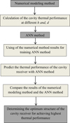Fig. 1

The procedure of determining the optimum structure of cavity receiver.

2 Models and description

2.1 General

The parabolic dish concentrator with a rectangular cavity receiver was used for absorbing the solar irradiation by the tube walls of the cavity receiver. The receiver presented in this work is a rectangular open-cavity receiver constructed with a coated copper tube through which the thermal oil flows (Fig. 2). The thermal oil as the solar working fluid was entered from the tube at the bottom of the receiver and the heated working fluid was exited from the tube at the top of the cavity receiver. The absorbed solar heat was transferred to the thermal oil. The receiver tube forms the inner wall of the open-cavity receiver.

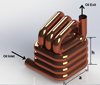Fig. 2

A square prismatic open-cavity solar receiver.

2.1.1 Receiver thermal modeling method

In this study, an accuracy thermal modeling method was applied based on the proposed method in [6]. In this method, the tubular cavity receiver was divided into a number of sections along the inner tube of the cavity receiver as following: 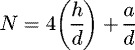$N = 4 (\frac{h}{d}) + \frac{a}{d}$ (1)

Then the surface temperature (T_s,n) and the net heat transfer rates () at different elements of the tube were determined by solving equations (2) and (3) using the Newton–Raphson method [6]: ${\dot{Q}}_{n e t, n} = \frac{(T_{s, n} - \sum_{i = 1}^{n - 1} (\frac{{\dot{Q}}_{n e t, i}}{{\dot{m}}_{o i l} c_{p 0}}) - T_{i n l e t, 0})}{(\frac{1}{h {A^{'}}_{n}} + \frac{1}{2 {\dot{m}}_{o i l} c_{p 0}})}$ (2) and ${\dot{Q}}_{n e t, n} = {\dot{Q}}_{n}^{*} - A_{n} ε_{n} σ (T_{s, n}^{4}) + A_{n} \sum_{j = 1}^{N} F_{n - j} ε_{j} σ (T_{s, n}^{4}) - A_{n} ε_{n} σ F_{n - \infty} T_{\infty}^{4} - A_{n} (m_{2} T_{s, n} + c_{2}) - \frac{A_{n}}{R_{c o n d}} (T_{s, n} - T_{\infty})$ (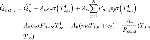3)

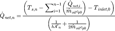
After calculation of the net heat gained () by each element tube along the tubular cavity receiver, the outlet temperature of the working fluid for each element tube can be calculated as following: 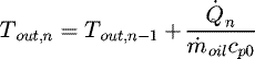$T_{o u t, n} = T_{o u t, n - 1} + \frac{{\dot{Q}}_{n}}{{\dot{m}}_{o i l} c_{p 0}}$ (4) where T_out,n is the outlet temperature of the working fluid for each element tube and T_out,n−1is the inlet temperature of the working fluid for it.

The collector efficiency was defined as following [15]: 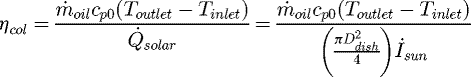$η_{c o l} = \frac{{\dot{m}}_{o i l} c_{p 0} (T_{o u t l e t} - T_{i n l e t})}{{\dot{Q}}_{s o l a r}} = \frac{{\dot{m}}_{o i l} c_{p 0} (T_{o u t l e t} - T_{i n l e t})}{(\frac{π D_{d i s h}^{2}}{4}) {\dot{I}}_{s u n}}$ (5) where T_inlet is the cavity inlet temperature of the working fluid that is assumed to be equal to 50 °C in this study and T_outlet is the cavity outlet temperature of the working fluid that is equal to the outlet temperature of the last element tube of the tubular cavity receiver.

The receiver surface temperature at different elements of the tube and the net heat transfer rate depend on the aperture size, the height of the cavity receiver, the mass flow rate of the solar working fluid, the receiver tube diameter and the working fluid inlet temperature. Thermal analyses parameters and their value are shown in Table 1. The thermal characteristics of the thermal Behran oil are obtained by [16].

Table 1

Thermal analysis parameters.

2.2 ANN description

ANNs are a simulation of the manner nerve cell (neurons) in the biological central nervous system. The important feature of the ANNs is that it could learn, memorize and create relationships among data [9]. The optimum weight of the network neurons was found by the ANN using recorded data and the output variables were predicted base on this optimum found weight of the network neurons [17]. In Figure 3, the method of the ANN output computing is illustrated.

In this study, ANN modeling was carried out in two stages. First, we applied the ANN approach for outlet temperature of the working fluid for each tube element. Second, the collector efficiencies as a thermal performance parameter of the cavity receiver were calculated (Eq. (5)) based on the predicted outlet temperature in the first stage for each condition prediction (Fig. 4). Figures 5 and 6 describe the details of the utilized ANN approach for h and d as the variable parameters, respectively. These figures illustrate the general methods for assuming of the training and evaluation values based on the numerical modeling results. It has to be mentioned that the numerical modeling results after validation with the experimental results were used for training and testing of ANN approach for different variable parameters.

In equation (6) the target value, o_j is the outcome of the ANN model. The parameter t_j stands for the estimated target from the ANN approach for an assumed input while o_j represents the desired target (i.e. measured data) from the similar input that has been generated by the setup. The R² value varies between 0 and +1. R² values near to +1 represent a robust positive linear correlation, while R² values near to 0 represent very weak correlation [19,20]. This value can be determined according to the below formula [21–28]: 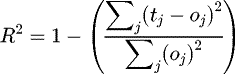$R^{2} = 1 - (\frac{\sum_{j} {(t_{j} - o_{j})}^{2}}{\sum_{j} {(o_{j})}^{2}})$ (6)

The network is trained by optimization and updating the weights for each node until the output gets as close as possible to the real target. The MSE of the network is given as [21–31]: $M S E = \frac{1}{2} \sum_{k = 1}^{G} \sum_{j = 1}^{m} {(o_{j} (k) - t_{j} (k))}^{2}$ (7)

Fig. 3

Output computing in ANN [18].

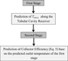Fig. 4

Stages of the ANN prediction of the collector performance for each considered variable parameter.

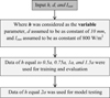Fig. 5

The procedure of the ANN method for the cavity depth as the variable.

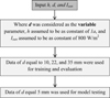Fig. 6

The procedure of the ANN method for the tube diameter as the variable.

3 Results and discussion

3.1 Validation of the numerical simulation with experimental results

It has to be mentioned that the numerical results were validated with the experimental results in [32]. The detail of the numerical method, results and validation of the results were explained in [32].

3.2 Comparing the ANN prediction with numerical results

3.2.1 Sensitivity analysis of the hidden neurons number

Before grappling with details of the gained results of the proposed intelligent based model, which called “ANN”, sensitivity analysis of the addressed model versus number of hidden neurons should be demonstrated. Figures 7 and 8 describe the effect of the number of hidden neurons in hidden layer of the developed network approach on the correlation coefficient (R²) and mean square error (MSE) of the proposed ANN model of the developed approach for the torque for the depth of the cavity and for the tube diameter as the variable, respectively. It can be seen from Figure 7 that the maximum correlation coefficient (R²) is gained when “hidden neurons ≥ 100” while the minimum correlation coefficient (R²) occurred when “hidden neurons = 1” and the minimum value of MSE occurred when “hidden neurons = 110” while maximum value of MSE is obtained when “hidden neurons = 1” in the ANN model for the depth of the cavity as the variable. Then it can be resulted that the optimum number of the hidden neurons for the depth of the cavity was found equal to 110,which has the maximum R² and minimum MSE. So hidden neurons equal to 110 will be applied for further analysis of the depth of the cavity as the variable.

While it can be seen from Figure 8 that the maximum correlation coefficient (R²) is gained when “hidden neurons = 30”, the minimum correlation coefficient (R²) occurred when “hidden neurons = 188”. One of the minimum values of MSE occurred when “hidden neurons = 30”, maximum value of MSE is obtained when “hidden neurons = 1” in the ANN model for the tube diameter as the variable. Then it can be resulted that the optimum number of the hidden neurons for the tube diameter as the variable was 30, which has the maximum R² and minimum MSE. So hidden neurons equal to 30 will be applied for further analysis of the tube diameter as the variable.

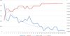Fig. 7

Variation of correlation coefficient and the MSE against number of hidden neurons for torque determination for the depth of the cavity as the variable.

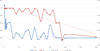Fig. 8

Variation of correlation coefficient and the MSE against number of hidden neurons for torque determination for the tube diameter as the variable.

3.2.2 Effect of the tube diameters

Figure 9 shows the accuracy of the ANN results compared to the numerical modeling results for the outlet temperature of the working fluid for each element along the inner tube of the cavity receiver in different tube diameters. Figure 9a depicts the accuracy of the ANN output compared to the numerical modeling results. Figure 9b displays a comparison of the ANN and the numerical modeling results of the outlet temperature of the working fluid along the inner tube of the cavity receiver.

It can be seen from Figure 9a and b that there is a good agreement with R² = 0.99 between the ANN results and the numerical modeling results for the outlet temperature of the working fluid for each element of the tubular cavity receiver.

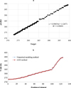Fig. 9

(a) Accuracy of ANN results compared with the numerical modeling results and (b) comparison of the ANN results and the numerical modeling results of the working fluid outlet temperature in different tube diameters.

3.2.3 Effect of the cavity depths

Figure 10 shows the accuracy of the ANN results compared to the numerical modeling results for the outlet temperature of the working fluid for each element along the inner tube of the cavity receiver in different cavity depths. Figure 10a depicts the accuracy of the ANN output compared to the numerical modeling results. Figure 10b displays a comparison of the ANN and the numerical modeling results of the outlet temperature of the working fluid along the inner tube of the cavity receiver.

It can be seen from Figure 10a and b that there is a good agreement with R² = 0.99 between the ANN results and the numerical modeling results for the outlet temperature of the working fluid for each element of the tubular cavity receiver.

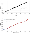Fig. 10

(a) Accuracy of ANN results compared with the numerical modeling results and (b) comparison of the ANN results and the numerical modeling results of the working fluid outlet temperature in different cavity depths.

3.2.4 Collector efficiency

Table 2 shows a comparison of the collector efficiency which was calculated by the thermal modeling method and predicted by the ANN method for d and h as the variable parameters. It can be resulted from Table 2 that the collector efficiency predicted by the ANN method can compare with the numerical modeling results. On the other hand, using the ANN method for prediction of the collector efficiency can save the time and cost for determining the optimum structure of the cavity receiver.

Table 2

Comparison of the collector efficiency calculated by the thermal modeling method and predicted by the ANN method.

4 Conclusion

The parabolic dish concentrator with a rectangular cavity receiver was investigated in this study. The dish concentrator diameter of 1.8 m with reflectivity of 84% and the rectangular cavity receiver with length of the aperture of 0.125 m were studied. The thermal oil was used as the working fluid. In this study, the performance of the cavity receiver was calculated in different methods such as a numerical modeling, based on the thermal modeling of the cavity receiver, and ANN method for the performance prediction. The purpose of this study was calculation of the optimum structure of the cavity receiver for achieving higher thermal performance by ANN approach as an accuracy approach with the less consumption of the cost and time. In the numerical modeling the performance of the cavity was calculated at the different depths, different diameter of tube, and different solar intensity. And the numerical modeling results were validated with experimental results. Then the resulted of the numerical modeling was used for training of the ANN method and finally prediction of the thermal performance of the cavity was conducted by this method. The main benefit of the ANN method was that the numerical modeling method saved the time and cost. The results obtained were as following:

there was a good agreement with R² = 0.99 between the predicted results of ANN and the calculated numerical modeling results for the outlet temperature of the working fluid for each tube element of the tubular cavity receiver, when the tube diameter and the cavity depth were investigated as the variable parameters;
the collector efficiency predicted by the ANN method can be compared to the numerical modeling results. On the other hand, using the ANN method for prediction of the collector efficiency can save the time and cost of the calculation for determining the optimum structure of the cavity receiver.

Nomenclature

a: aperture length, m

A: area, m²

Á: area ratio (A_ap/A_conc)

C: aspect ratio

_Ć: optimum aspect ratio

c_p: constant pressure specific heat, J kg⁻¹ K⁻¹

d: receiver tube diameter, m

F: view factor

h: cavity depth, m

I: direct normal solar irradiance, W m⁻²

k: thermal conductivity, W m⁻¹ K⁻¹

: net heat transfer rate, W

: rate of available solar heat at dish concentrator, W

: system mass flow rate, kg s⁻¹

R: thermal resistance, K W⁻¹

T: temperature, K

t: thickness, m

Greek symbols

ε: emissivity

σ: Stefan–Boltzmann constant, W m⁻² K⁻⁴

ρ: density, kg m⁻³

η: efficiency

Subscripts

0: initial inlet to receiver

ap: aperture

col: overall for the collector

dish: dish concentrator

f: fluid

inlet: at the inlet

ins: insulation

n: tube section number

s: surface

outlet: at the outlet

total: total

∞: environment

References

S.A. Kalogirou, Solar thermal collectors and applications, Prog. Energy Combust. 30 (2004) 231–295 [Google Scholar]
J.A. Harris, T.G. Lenz, Thermal performance of solar concentrator/cavity receiver systems, Solar Energy 34 (1985) 135–142 [CrossRef] [Google Scholar]
A.M. Clausing, An analysis of convective losses from cavity solar central receiver, Solar Energy 27 (1981) 295–300 [CrossRef] [Google Scholar]
P. Le Quere, F. Penot, M. Mirenayat, Experimental study of heat loss through natural convection from an isothermal cubic open cavity, Sandia Laboratory Report, 1981, SAN D81-8014 [Google Scholar]
W. Huang, F. Huang, P. Hu, Z. Chen, Prediction and optimization of the performance of parabolic solar dish concentrator with sphere receiver using analytical function, Renew. Energy 53 (2013) 18–26 [CrossRef] [Google Scholar]
W.G. Le Roux, T. Bello-Ochende, J.P. Meyer, The efficiency of an open-cavity tubular solar receiver for a small-scale solar thermal Brayton cycle, Energy Convers. Manag. 84 (2014) 457–470 [CrossRef] [Google Scholar]
S.A. Kalogirou, C.C. Neocleous, C.N. Schizas, Artificial neural networks in modeling the heat-up response of a solar steam generation plant, in: Proceedings of the International Conference EANN'96, 1996, pp. 1–4 [Google Scholar]
S.A. Kalogirou, S. Panteliou, A. Dentsoras, Modeling of solar domestic water heating systems using artificial neural networks, Solar Energy 65 (1999) 335–342 [CrossRef] [Google Scholar]
S.A. Kalogirou, Artificial neural networks in renewable energy systems applications: a review, Renew. Sustain. Energy Rev. 5 (2001) 373–401 [Google Scholar]
A. Sözen, T. Menlik, S. Ünvar, Determination of efficiency of flat-plate solar collectors using neural network approach, Exp. Syst. Appl. 35 (2008) 1533–1539 [CrossRef] [Google Scholar]
S.A. Kalogirou, Artificial neural networks and genetic algorithms for the modeling, simulation, and performance prediction of solar energy systems, in: Assessment and simulation tools for sustainable energy systems, Green Energy and Technology, Vol. 129, Chapter 7, 2013, pp. 225–245 [CrossRef] [Google Scholar]
W. Yaïci, E. Entchev, Performance prediction of a solar thermal energy system using artificial neural networks, Appl. Therm. Eng. 73 (2014) 1348–1359 [CrossRef] [Google Scholar]
S.A. Kalogirou, E. Mathioulakis, V. Belessiotis, Artificial neural networks for the performance prediction of large solar systems, Renew. Energy 63 (2014) 90–97 [CrossRef] [Google Scholar]
S. Amirkhani, Sh. Nasirivatan, A.B. Kasaeian, A. Hajinezhad, ANN and ANFIS models to predict the performance of solar chimney power plants, Renew. Energy 83 (2015) 597–607 [CrossRef] [Google Scholar]
Y.A. Cengel, Heat and mass transfer, 3rd ed., McGraw-Hill, Nevada, 2006 [Google Scholar]
A. Baghernejad, M. Yaghoubi, Thermoeconomic methodology of analysis and optimization of a hybrid solar thermal power plant, Int. J. Green Energy 10 (2013) 588–609 [CrossRef] [Google Scholar]
S.A. Kalogirou, Applications of artificial neural networks for energy systems, Appl. Energy 67 (2000) 17–35 [CrossRef] [Google Scholar]
A.K. Tripathy, S. Mohapatra, S. Beura, G. Pradhan, Weather forecasting using ANN and PSO, Int. J. Scient. Eng. Res. 2 (2011) 1–5 [Google Scholar]
Y.O. Ozgoren, S. Cetinkaya, S. Sarıdemir, A. Cicek, F. Kara, Predictive modeling of performance of a helium charged Stirling engine using an artificial neural network, Energy Convers. Manage. 67 (2013) 357–368 [CrossRef] [Google Scholar]
C. Sayin, H.M. Ertunc, M. Hosoz, I. Kilicaslan, M. Canakci, Performance and exhaust emissions of a gasoline engine using artificial neural network, Appl. Therm. Eng. 27 (2007) 46–54 [CrossRef] [Google Scholar]
K. Hornick, M. Stinchcombe, H. White, Neural Network 2 (1989) 359–366 [CrossRef] [Google Scholar]
M. Brown, C. Harris, Neural fuzzy adaptive modeling and control, Prentice-Hall, Englewood Cliffs, NJ, 1994 [Google Scholar]
S. Zendehboudi, M.A. Ahmadi, A. Bahadori, A. Shafiei, T. Babadagli, A developed smart technique to predict minimum miscible pressure − EOR implication, Canad. J. Chem. Eng. 91 (2013) 1–13 [Google Scholar]
S. Zendehboudi, M.A. Ahmadi, O. Mohammadzadeh, A. Bahadori, I. Chatzis, Thermodynamic investigation of asphaltene precipitation during primary oil production, laboratory and smart technique, Ind. Eng. Chem. Res., 2017, doi: 10.1021/ie301949c [Google Scholar]
M.H. Ahmadi, S.S. Ghare Aghaj, A. Nazeri, Prediction of power in solar Stirling heat engine by using neural network based on hybrid genetic algorithm and particle swarm optimization, Neural Comput. Appl. 22 (2013) 1141–1150 [CrossRef] [Google Scholar]
M.H. Ahmadi, M.A. Ahmadi, S.A. Sadatsakkak, M. Feidt, Connectionist intelligent model estimates output power and torque of Stirling engine, Renew. Sustain. Energy Rev. 50 (2015) 871–883 [CrossRef] [Google Scholar]
M.H. Ahmadi, M.A. Ahmadi, M. Mehrpooya, M.A. Rosen, Using GMDH neural networks to model the power and torque of a Stirling engine, Sustainability 7 (2015) 2243–2255 [CrossRef] [Google Scholar]
S.M. Pourkiaei, M.H. Ahmadi, S.M. Hasheminejad, Modeling and experimental verification of a 25W fabricated PEM fuel cell by parametric and GMDH-type neural network, Mech. Indust. 17 (2016) 105 [CrossRef] [EDP Sciences] [Google Scholar]
S.A. Sadatsakkak, M.H. Ahmadi, M.A. Ahmadi, Implementation of artificial neural-networks to model the performance parameters of Stirling engine, Mech. Indust. 17 (2016) 307 [CrossRef] [EDP Sciences] [Google Scholar]
M.H. Ahmadi, M.A. Ahmadi, M. Ashouri, F.R. Astaraei, R. Ghasempour, F. Aloui, Prediction of performance of Stirling engine using least squares support machine technique, Mech. Indust. 17 (2016) 506 [CrossRef] [EDP Sciences] [Google Scholar]
A. Kasaeian, M. Mehrpooya, M. Aghaie, M.H. Ahmadi, Solar radiation prediction based on ICA and HGAPSO for Kuhin City, Iran, Mech. Indust. 17 (2016) 509 [CrossRef] [EDP Sciences] [Google Scholar]
R. Loni, A.B. Kasaeian, E.A. Asli-Ardeh, B. Ghobadian, W.G. Le Roux, Performance study of a solar-assisted organic Rankine cycle using a dish mounted rectangular-cavity tubular solar receiver, Appl. Therm. Eng. 108 (2016) 1298–1309 [CrossRef] [Google Scholar]

Cite this article as: R. Loni, A. Kasaeian, K. Shahverdi, E. Askari Asli-Ardeh, B. Ghobadian, M.H. Ahmadi, ANN model to predict the performance of parabolic dish collector with tubular cavity receiver, Mechanics & Industry 18, 408 (2017)

All Tables

Table 1

Thermal analysis parameters.

In the text

Table 2

Comparison of the collector efficiency calculated by the thermal modeling method and predicted by the ANN method.

In the text

All Figures

	Fig. 1 The procedure of determining the optimum structure of cavity receiver.
In the text

	Fig. 2 A square prismatic open-cavity solar receiver.
In the text

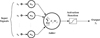	Fig. 3 Output computing in ANN [18].
In the text

	Fig. 4 Stages of the ANN prediction of the collector performance for each considered variable parameter.
In the text

	Fig. 5 The procedure of the ANN method for the cavity depth as the variable.
In the text

	Fig. 6 The procedure of the ANN method for the tube diameter as the variable.
In the text

	Fig. 7 Variation of correlation coefficient and the MSE against number of hidden neurons for torque determination for the depth of the cavity as the variable.
In the text

	Fig. 8 Variation of correlation coefficient and the MSE against number of hidden neurons for torque determination for the tube diameter as the variable.
In the text

	Fig. 9 (a) Accuracy of ANN results compared with the numerical modeling results and (b) comparison of the ANN results and the numerical modeling results of the working fluid outlet temperature in different tube diameters.
In the text

	Fig. 10 (a) Accuracy of ANN results compared with the numerical modeling results and (b) comparison of the ANN results and the numerical modeling results of the working fluid outlet temperature in different cavity depths.
In the text

Current usage metrics show cumulative count of Article Views (full-text article views including HTML views, PDF and ePub downloads, according to the available data) and Abstracts Views on Vision4Press platform.

Data correspond to usage on the plateform after 2015. The current usage metrics is available 48-96 hours after online publication and is updated daily on week days.

Initial download of the metrics may take a while.

[1] S.A. Kalogirou, Solar thermal collectors and applications, Prog. Energy Combust. 30 (2004) 231–295 [Google Scholar]

[2] J.A. Harris, T.G. Lenz, Thermal performance of solar concentrator/cavity receiver systems, Solar Energy 34 (1985) 135–142 [CrossRef] [Google Scholar]

[3] A.M. Clausing, An analysis of convective losses from cavity solar central receiver, Solar Energy 27 (1981) 295–300 [CrossRef] [Google Scholar]

[4] P. Le Quere, F. Penot, M. Mirenayat, Experimental study of heat loss through natural convection from an isothermal cubic open cavity, Sandia Laboratory Report, 1981, SAN D81-8014 [Google Scholar]

[5] W. Huang, F. Huang, P. Hu, Z. Chen, Prediction and optimization of the performance of parabolic solar dish concentrator with sphere receiver using analytical function, Renew. Energy 53 (2013) 18–26 [CrossRef] [Google Scholar]

[6] W.G. Le Roux, T. Bello-Ochende, J.P. Meyer, The efficiency of an open-cavity tubular solar receiver for a small-scale solar thermal Brayton cycle, Energy Convers. Manag. 84 (2014) 457–470 [CrossRef] [Google Scholar]

[7] S.A. Kalogirou, C.C. Neocleous, C.N. Schizas, Artificial neural networks in modeling the heat-up response of a solar steam generation plant, in: Proceedings of the International Conference EANN'96, 1996, pp. 1–4 [Google Scholar]

[8] S.A. Kalogirou, S. Panteliou, A. Dentsoras, Modeling of solar domestic water heating systems using artificial neural networks, Solar Energy 65 (1999) 335–342 [CrossRef] [Google Scholar]

[9] S.A. Kalogirou, Artificial neural networks in renewable energy systems applications: a review, Renew. Sustain. Energy Rev. 5 (2001) 373–401 [Google Scholar]

[10] A. Sözen, T. Menlik, S. Ünvar, Determination of efficiency of flat-plate solar collectors using neural network approach, Exp. Syst. Appl. 35 (2008) 1533–1539 [CrossRef] [Google Scholar]

[11] S.A. Kalogirou, Artificial neural networks and genetic algorithms for the modeling, simulation, and performance prediction of solar energy systems, in: Assessment and simulation tools for sustainable energy systems, Green Energy and Technology, Vol. 129, Chapter 7, 2013, pp. 225–245 [CrossRef] [Google Scholar]

[12] W. Yaïci, E. Entchev, Performance prediction of a solar thermal energy system using artificial neural networks, Appl. Therm. Eng. 73 (2014) 1348–1359 [CrossRef] [Google Scholar]

[13] S.A. Kalogirou, E. Mathioulakis, V. Belessiotis, Artificial neural networks for the performance prediction of large solar systems, Renew. Energy 63 (2014) 90–97 [CrossRef] [Google Scholar]

[14] S. Amirkhani, Sh. Nasirivatan, A.B. Kasaeian, A. Hajinezhad, ANN and ANFIS models to predict the performance of solar chimney power plants, Renew. Energy 83 (2015) 597–607 [CrossRef] [Google Scholar]

[15] Y.A. Cengel, Heat and mass transfer, 3rd ed., McGraw-Hill, Nevada, 2006 [Google Scholar]

[16] A. Baghernejad, M. Yaghoubi, Thermoeconomic methodology of analysis and optimization of a hybrid solar thermal power plant, Int. J. Green Energy 10 (2013) 588–609 [CrossRef] [Google Scholar]

[17] S.A. Kalogirou, Applications of artificial neural networks for energy systems, Appl. Energy 67 (2000) 17–35 [CrossRef] [Google Scholar]

[18] A.K. Tripathy, S. Mohapatra, S. Beura, G. Pradhan, Weather forecasting using ANN and PSO, Int. J. Scient. Eng. Res. 2 (2011) 1–5 [Google Scholar]

[19] Y.O. Ozgoren, S. Cetinkaya, S. Sarıdemir, A. Cicek, F. Kara, Predictive modeling of performance of a helium charged Stirling engine using an artificial neural network, Energy Convers. Manage. 67 (2013) 357–368 [CrossRef] [Google Scholar]

[20] C. Sayin, H.M. Ertunc, M. Hosoz, I. Kilicaslan, M. Canakci, Performance and exhaust emissions of a gasoline engine using artificial neural network, Appl. Therm. Eng. 27 (2007) 46–54 [CrossRef] [Google Scholar]

[21] K. Hornick, M. Stinchcombe, H. White, Neural Network 2 (1989) 359–366 [CrossRef] [Google Scholar]

[22] M. Brown, C. Harris, Neural fuzzy adaptive modeling and control, Prentice-Hall, Englewood Cliffs, NJ, 1994 [Google Scholar]

[23] S. Zendehboudi, M.A. Ahmadi, A. Bahadori, A. Shafiei, T. Babadagli, A developed smart technique to predict minimum miscible pressure − EOR implication, Canad. J. Chem. Eng. 91 (2013) 1–13 [Google Scholar]

[24] S. Zendehboudi, M.A. Ahmadi, O. Mohammadzadeh, A. Bahadori, I. Chatzis, Thermodynamic investigation of asphaltene precipitation during primary oil production, laboratory and smart technique, Ind. Eng. Chem. Res., 2017, doi: 10.1021/ie301949c [Google Scholar]

[25] M.H. Ahmadi, S.S. Ghare Aghaj, A. Nazeri, Prediction of power in solar Stirling heat engine by using neural network based on hybrid genetic algorithm and particle swarm optimization, Neural Comput. Appl. 22 (2013) 1141–1150 [CrossRef] [Google Scholar]

[26] M.H. Ahmadi, M.A. Ahmadi, S.A. Sadatsakkak, M. Feidt, Connectionist intelligent model estimates output power and torque of Stirling engine, Renew. Sustain. Energy Rev. 50 (2015) 871–883 [CrossRef] [Google Scholar]

[27] M.H. Ahmadi, M.A. Ahmadi, M. Mehrpooya, M.A. Rosen, Using GMDH neural networks to model the power and torque of a Stirling engine, Sustainability 7 (2015) 2243–2255 [CrossRef] [Google Scholar]

[28] S.M. Pourkiaei, M.H. Ahmadi, S.M. Hasheminejad, Modeling and experimental verification of a 25W fabricated PEM fuel cell by parametric and GMDH-type neural network, Mech. Indust. 17 (2016) 105 [CrossRef] [EDP Sciences] [Google Scholar]

[29] S.A. Sadatsakkak, M.H. Ahmadi, M.A. Ahmadi, Implementation of artificial neural-networks to model the performance parameters of Stirling engine, Mech. Indust. 17 (2016) 307 [CrossRef] [EDP Sciences] [Google Scholar]

[30] M.H. Ahmadi, M.A. Ahmadi, M. Ashouri, F.R. Astaraei, R. Ghasempour, F. Aloui, Prediction of performance of Stirling engine using least squares support machine technique, Mech. Indust. 17 (2016) 506 [CrossRef] [EDP Sciences] [Google Scholar]

[31] A. Kasaeian, M. Mehrpooya, M. Aghaie, M.H. Ahmadi, Solar radiation prediction based on ICA and HGAPSO for Kuhin City, Iran, Mech. Indust. 17 (2016) 509 [CrossRef] [EDP Sciences] [Google Scholar]

[32] R. Loni, A.B. Kasaeian, E.A. Asli-Ardeh, B. Ghobadian, W.G. Le Roux, Performance study of a solar-assisted organic Rankine cycle using a dish mounted rectangular-cavity tubular solar receiver, Appl. Therm. Eng. 108 (2016) 1298–1309 [CrossRef] [Google Scholar]