| Issue |
Mechanics & Industry
Volume 21, Number 4, 2020
|
|
|---|---|---|
| Article Number | 406 | |
| Number of page(s) | 11 | |
| DOI | https://doi.org/10.1051/meca/2020027 | |
| Published online | 06 May 2020 | |
Regular Article
Rotational speed control of magnetic coupling with variable damping method
1
College of Mechanical and Electrical Engineering, Nanjing University of Aeronautics and Astronautics, Nanjing 210016,
PR China
2
National Key Laboratory of Science and Technology on Helicopter Transmission, Nanjing University of Aeronautics and Astronautics, Nanjing 210016, PR China
3
National Deep Sea Center, Qingdao 266237, PR China
* e-mail: This email address is being protected from spambots. You need JavaScript enabled to view it.
Received:
19
September
2019
Accepted:
23
March
2020
Abstract
Permanent Magnetic Coupling (PMC) is used in underwater vehicle to transmit torque from the motor to propeller without leakage and friction. Output rotational speed stability of PMC is an important index indicating the PMC output makes smaller vibration. To improve the stability of the output rotational speed, PMC dynamic characteristic was analyzed based on Lagrange equation in this paper. The dynamic characteristic was indicated by the angular phase generated by the master rotor and the slave rotor. The angular phase varied with the damping coefficient, torsional rigidity and rotational inertia of PMC. These parameters' influence on the angular phase was analyzed and the results revealed the rules between these parameters and the angular phase. Based on the rules, a variable damping method was proposed to control the angular phase. The angular phase changed smoothly with this method that was used to design a variable damping controller based on electromagnetic damping effect principle. This method was verified by theoretical calculation and finite element analysis (FEA). Finally, a novel variable damping PMC was designed to improve the output rotational speed stability of PMC.
Key words: Permanent magnetic coupling / output speed stability / variable damping method / angular phase / optimization
© AFM, EDP Sciences 2020
1 Introduction
Ocean covers about 70% of the earth surface. It possesses abundant resources and provides us with innumerable benefits. Humans have invented various machines to study the ocean like underwater vehicle. In the past few decades, ocean exploration technology has been developed rapidly [1]. The propulsor is the power source of the underwater vehicle. Many experts and scholars do a lot of studies on it [2–4]. Some novel propulsors have been designed [5,6]. Despite recent progress, some problems still remain when the propulsor is used in underwater vehicles [7]. As we all known, the propeller and motor should be sealed with sealing ring. Propeller shaft will wear the sealing ring, so some complex sealed system and wear-resistant material have been studied [8–11]. This paper mainly analyzes and optimizes the transmission mechanism between the propeller and motor to improve propulsor's dependability and life-span.
Permanent Magnetic Coupling (PMC) is a non-contact, flexible and isolated transmission component [12–14]. It is used in propulsor to isolate the motor from seawater and avoid leakage [15] as shown in Figure 1a. Propulsor with PMC have many merits than those with traditional mechanical contact devices. At the start-up of PMC, the angular phase between the master rotor and the slave rotor will appear as shown in Figure 1b. Then magnets on the rotors will generate tangential force, then the torque from the master rotor is transmitted to the slave rotor. At appropriate range of the angular phase, PMC can perform best. PMC structural parameters cannot change once PMC is manufactured, so the appropriate structural parameters should be determined when PMC is designed.
Magnetic force generates the torque which causes speed ripple and torsion oscillation on the slave rotor during startup stage. If speed ripple and torsion oscillation-which can be indicated by the angular phase-are serious, they will affect propulsor performance and even make propulsor fail to work. Stable speed and small torsion oscillation which are influenced by structural parameters, input torque, load and installation precision are vital to improve propulsor performance.
Lagrange equation is usually used to analyze dynamic characteristics of mechanism [16–18]. It can analyze different parameters' influence on the dynamic characteristics by defining generalized force and generalized coordinates which allow us to easily carry out parametric studies and optimization. Dynamic equations derived from Lagrange equation can avoid constraint reaction and reduce solving difficulty, it is an effective method to analyze PMC.
This paper has three main objectives. First, the dynamic equations of PMC were built based on the Lagrange equation, and the angular phase between the master rotor and the slave rotor were chosen as the index to analyze the output speed stability which was a basic dynamic characteristic of PMC. Then, the influence of structural parameters on the output speed stability was analyzed, considering damping coefficient, torsional rigidity and rotational inertia. Eventually, according to the parameters' influence on the output speed stability of PMC, a control method was proposed to control the output speed stability and a novel PMC controller was designed based on electromagnetic damping effect principle. In general, the paper provided a new method to optimize PMC which could improve propulsor's dependability and life-span.
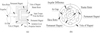 |
Fig. 1 Permanent magnetic coupling. (a) The application of PMC; (b) angular phase in PMC. |
2 Mathematical model
The Lagrange equation that the dissipation term is part of generalized force is expressed as follows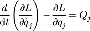 (1)
(1)
 (2)
(2)
where qj is generalized coordinates,  is the generalized velocity, T is the kinetic energy, U is the potential energy, Qj is the generalized force.
2.1 PMC structural parameters
Once PMC is installed, the installation deviations and the assembly gap have already existed, including axial deviation, radial deviation and angle deviation. The axial deviation and the assembly gap have little impact on the dynamic characteristic when a machine works, so the radial and angle deviations need to be considered. As shown in Figure 2, assuming that the geometric center O1 coordinates of the master rotor are (x1, y1), the geometric center O2 coordinates of the slave rotor are (x2, y2), the radial deviation of the slave rotor is d, the angle deviation of the slave rotor is ϕ, the distance from O2 to the supporting point is l, the rotation angle of the slave rotor is α. Then according to geometric relations, x2 and y2 can be written as (3)
(3)
 (4)
(4)
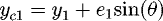
When PMC is manufactured, center-of-mass deviation exists in the master rotor and slave rotor. Assuming that the center-of-mass deviation of the master rotor is e1, the center-of-mass deviation of the slave rotor is e2; the rotation angle of the master rotor is θ. The center-of-mass coordinates of the master rotor are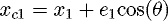 (5)
(5)
 (6)
(6)
The center-of-mass coordinates of the slave rotor are (7)
(7)
 (8)
(8)
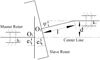 |
Fig. 2 PMC structural parameters. |
2.2 Kinetic energy
The kinetic energy T of PMC consists of translational kinetic energy TDP and rotational kinetic energy TDZ of the master rotor and the slave rotor, as following: (9)
(9)
 (10)
(10)
 (11)
(11)
where m1 is the mass of the master rotor, m2 is the mass of the slave rotor, vc1 is translational velocity of the master rotor, vc2 is the translational velocity of the slave rotor, J1 is the rotational inertia of the master rotor, J2 is the rotational inertia of the slave rotor. Then based on velocity composition law, velocity can be expressed as (12)
(12)
 (13)
(13)
2.3 Potential energy
Because the magnetic force is used to transmit the torque, potential energy exists in the magnetic field which generates the magnetic force. PMC can be simplified as a spring coupling as shown in Figure 3. The spring stiffness is k(θ) and equals the torsional rigidity of PMC, so k(θ) can be written as (14)
(14)
where M is the torque applied on PMC, Δθ is angular phase between the master rotor and slave rotor.
The potential energy U1 in magnetic field is (15)
(15)
The elastic potential energy U2 between supporting structures and the shaft is (16)
(16)
where k1 is the elastic stiffness of input, k2 is the elastic stiffness of output.
The potential energy U of PMC is (17)
(17)
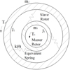 |
Fig. 3 PMC simplified model. |
2.4 Kinetic equations
When PMC is running, the master rotor is applied with input torque T1 and damping force  , as the slave rotor is applied with load torque T2 and damping force. These torques and forces are non-potential generalized force, so Qj is
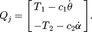 (18)
(18)
To analyze the response characteristics between the slave rotor and the master rotor, θ and α are chosen as generalized coordinates. Assuming that k(θ) is a constant K, then the kinetic equations of PMC can be derived from the Lagrange equation according to equations (1)–(18), as following,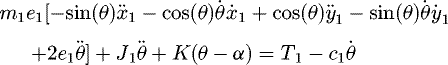 (19)
(19)
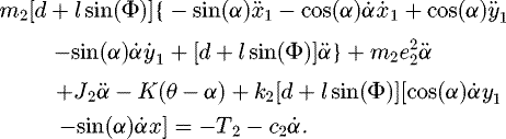 (20)
(20)
Usually, the geometric center coordinates O1 of the master rotor are fixed and x1, y1 are constant, so the kinetic equations can be expressed as (21)
(21)
 (22)
(22)
According to equation (22), the radial deviation d, the angle deviation Φ and the center-of-mass deviation e2 have the similar effect with increasing the rotational inertia of the slave rotor, so a total rotational inertia J can be written as (23)
(23)
3 Results and discussion
3.1 Relationship between torsional rigidity and angular phase
Because the relationship between torque and angular phase is nonlinear, it is difficult to calculate theoretical torsional rigidity. To obtain this relationship, a prototype experiment was carried out as shown in Figure 4. The electromotor drove the PMC by the master rotor and the magnetic powder brake kept the slave rotor still. Thus the torque applied on the master rotor and the rotating angle was measured by a torque-speed sensor. The measurement precision was improved by averaging the testing values.
Some measured data was listed in Table 1. The relation curve of torque T and angular phase Δθ was illustrated in Figure 5, and the fitting formula was obtained as equation
(24). According to the derivative of equation (24), the relationship between torsional rigidity k(θ) and angular phase Δθ was obtained as shown in equation (25) and Figure 6
.
 (24)
(24)
 (25)
(25)
As shown in Figure 6, maximum torsional rigidity is 51.72 Nm/rad and the start-up torsional rigidity is about 40 Nm/rad. Because torsional rigidity cannot be negative, the optimal range of the angular phase is 0–0.2 rad, and torsional rigidity distributes mainly in 20–51.72 Nm/rad.
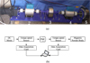 |
Fig. 4 Prototype. (a) Test rig: 1. DC Motor, 2. Torque-speed Sensor, 3. PMC, 4. Torque-speed Sensor, 5. Magnetic Powder Brake. (b) Schematic diagram of the test rig. |
Measured data of torque and angular phase.
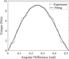 |
Fig. 5 Relationship between torque and angular phase. |
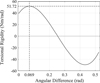 |
Fig. 6 Relationship between torsional rigidity and angular phase. |
3.2 Angular phase calculation
The slave rotor was connected to the load like the generator. The experiment showed that a certain damping relation existed between load torque T2 and angular velocity  . Assuming damping coefficient was Cd, then T2 could be expressed as
 (26)
(26)
Then transfer function G(s) between α and θ was derived from equation (22) as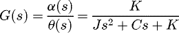 (27)
(27)
where C = C2+Cd, which meant the damping effect of output.
In the experiment, rotation speed was always invariable, so the rotation angle of the master rotor increased linearly with time. Assuming that the master rotor angular velocity was 1 rad/s, when PMC dynamic characteristics were analyzed, it meant the unit ramp input function was used to simulate the working state. Then the Laplace function of the slave rotor rotation angle could be expressed as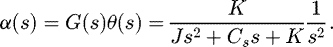 (28)
(28)
The angular phase and its variation were important indexes to indicate the output speed stability of PMC [13,19]. The smooth variation of the angular phase meant that the slave rotor could follow the master rotor steadily [20]. The small angular phase indicated that the slave rotor is closer to the master rotor and PMC would transmit a bigger torque [21]. Angular phase is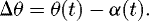 (29)
(29)
By actual measurement and calculation, some parameters were got: J = 0.17 kg m2, C2 = 0.1616 Nm s/rad, Cd = 1.21 Nm · s/rad. Based on Figure 6, the torsional rigidity was set as 45 Nm/rad. The above parameters were reference values to analyze the dynamic characteristics of PMC.
3.3 Output speed stability analysis
Once PMC is manufactured, the rotational inertia and torsional rigidity are fixed and the only variable parameter is damping coefficient. Damping coefficient which was set as C = 0.1, 0.5, 1, 1.5, 2.5, 3.5, 5 Nm s/rad was used to analyze the variation of the angular phase. Figure 7 shows the relationships between the angular phase Δθ and different damping coefficients C.
From Figure 7, when damping coefficient is less than 1.5 Nm s/rad, angular phase oscillates, whereas the variation of the angular phase is very smooth when damping coefficient is more than 3.5 Nm s/rad. That means small damping coefficient causes the oscillation of angular phase while big damping coefficient can stabilize the variation. As time passed, angular phase tends to be a stable value which changes with damping coefficient. With damping coefficient rising, the start-up oscillation will disappear and angular phase stable value will increase.
In the above analysis, the rotational inertia and the torsional rigidity were constant. Here they are changed to analyze the variation of the angular phase with different damping coefficients . K = 45 Nm/rad, J = 0.1, 0.25 kg m2 are set and Figure 8 shows the relationship between angular phase and damping coefficient with different rotational inertia. J = 0.17 kg m2, K = 5, 60 Nm/rad are set and Figure 8 Relationship between angular phase and damping coefficient with different rotational inertia.
Figure 9 shows the relationship between angular phase and damping coefficient with different torsional rigidity.
From Figures 7 and 8, the rotational inertia has no impact on the stable value of the angular phase, whereas the angular phase oscillates seriously with the rotational inertia increasing. For example, when C = 0.1 Nm s/rad, the maximum oscillation amplitude is about 0.04, 0.06, 0.08 rad for J = 0.1, 0.17, 0.25 kg m2, respectively. It means that a large rotational inertia is harmful to the output speed stability of PMC.
From Figures 7 and 9, the variation of angular phase is smoother with K = 5 Nm/rad than K = 60 Nm/rad, while the stable value is bigger. That means the smaller the torsional rigidity is, the smaller angular phase fluctuates. That benefits the output speed stability of PMC, but will make a larger stable value or even make angular phase out of the optimal range.
From Figures 7–9, the rotational inertia and torsional rigidity have no effect on the variation tendency of the angular phase with different damping coefficients. Big damping coefficient is good for the smooth variation of the angular phase, but it results in a large stable value. Though small damping coefficient can get small stable value, it causes oscillation.
To describe the influence of rotational inertia and torsional rigidity clearly, the following analysis was conducted. Figure 10 shows the relationship between angular phase and different rotational inertia when C = 1.37 Nm s/rad, K = 45 Nm/rad, J = 0.02, 0.05, 0.1, 0.15, 0.2 kg m2. Figure 11 shows the relationships between angular phase and different torsional rigidities when C = 1.37 Nm s/rad, J = 0.17 kg m2, K = 5, 10, 15, 30, 45, 60 Nm/rad.
From Figure 10, the stable value of the angular phase is above 0.03 rad and has nothing with the rotational inertia. However, high rotational inertia causes more serious oscillation than the smaller one. From Figure 11, the bigger the torsional rigidity is, the smaller the stable value is, but the oscillation is more serious. Figures 10 and 11 further validate the influence of rotational inertia and torsional rigidity on angular phase, and they support the above analysis.
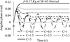 |
Fig. 7 Relationship between angular phase and damping coefficient. |
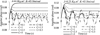 |
Fig. 8 Relationship between angular phase and damping coefficient with different rotational inertia. |
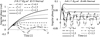 |
Fig. 9 Relationship between angular phase and damping coefficient with different torsional rigidity. |
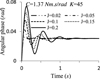 |
Fig. 10 Relationships between angular phase and different rotational inertias. |
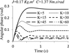 |
Fig. 11 Relationships between angular phase and different torsional rigidities. |
3.4 Output speed stability optimization
According to the above analyses, the big damping coefficient can help get smoother variation and bigger stable value of angular phase. Based on the variation of the angular phase, the running process of PMC involves four stages: start-up, separation, oscillation, and stabilization, as shown in Figure 12. In start-up (0–0.1 s), damping coefficient has no impact on the angular phase variation. In separation (0.1–0.2 s), the angular phase varies with different damping coefficients. In oscillation (0.2–0.9 s), the small damping coefficient causes the oscillation but the big damping coefficient makes angular phase stable. In stability (0.9 s∼), the angular phase tends to be stable. So when PMC begins to work, it can be set that the damping coefficient keeps a small value in start-up, next increasing to the maximum in the separation. Then the damping coefficient decreases to a stable value in oscillation and keeps the value in the stabilization. This is the method to achieve the smooth variation of the angular phase and keep the angular phase in the optimal range. Figure 13 is a variable damping coefficient curve which was used to control PMC. Based on the above analysis, start-up damping coefficient, maximum damping coefficient and stabilization damping coefficient were set as 0.1, 5, 1.4 Nm s/rad, respectively. The time of start-up, separation, oscillation and stabilization were 0–0.1 s, 0.1–0.2 s, 0.2–1.4 s, 1.4 s ∼, respectively.
Equation (25) reveals that the torsional rigidity changes with the angular phase, so the variation of torsional rigidity should be considered when the variable damping coefficient curve is used. PMC dynamic characteristic can be analyzed by iterative computation according to equations (25), (29) and Figure 13. Torsional rigidity K initial value was 40 Nm/rad according to Figure 6, damping coefficient C initial value was 0.1 Nm s/rad according to Figure 13, and rotational inertia J was constant. Time step was set as 0.001 s, and the smaller time step was, the more precise the result would be. Taking initial values of K, C, J into equation (29), initial angular phase was got. Then according to the initial angular phase and equation (29), the torsional rigidity could be got and the damping coefficient could be got from Figure 13. Step by step like this, the variation of the angular phase was calculated. Figure 14 shows the relationship between angular phase and rotational inertia with variable damping coefficient and Figure 15 shows the relationship between torsional rigidity and rotational inertia with variable damping coefficient.
Figure 14 shows that the variation of the angular phase has almost nothing with rotational inertia except in oscillation stage, and angular phase stable value close to 0.03 rad. In oscillation stage, the angular phase maximum values appear, and their difference is less than 0.05 rad with J increasing from 0.05 to 0.4 kg m2. From Figure 15, the torsional rigidity shows the same characteristic and the stable value of the angular phase close 45 Nm/rad. In oscillation stage, the minimum values appear, and their difference is about 15 Nm/rad. Figures 14 and 15 indicate that angular phase and torsional rigidity vary smoothly and their stable values are in optimal range.
To further study the influence of the variable damping coefficients on angular phase and torsional rigidity, the maximum damping coefficient in Figure 13 was set as C_M = 2, 3, 5, 7 Nm s/rad, J = 0.17 kg m2. By calculation, relationships between angular phase and different maximum damping coefficients are shown in Figure 16 and the relationships between torsional rigidity and different maximum damping coefficients are shown in Figure 17.
Figure 16 shows that the maximum angular phase of C_M = 2 Nm s/rad is less than the others, but C_M = 2 Nm s/rad causes oscillation compared with C_M = 3, 5, 7 Nm s/rad. The maximum angular phase is large with big C_M, such as C_M = 7 Nm s/rad is larger 0.1 rad than C_M = 2 Nm s/rad. Figure 17 shows that C_M = 2 Nm s/rad has a better torsional rigidity range than the others, and the minimum value is about 22 Nm/rad, that is beneficial to improve the rigidity of PMC. However, negative rigidity will appear with bigger C_M, such as C_M = 5, 7 Nm s/rad, that is harmful to the output speed stability of PMC. In summary, the big C_M will cause the negative torsional rigidity and the small C_M will cause the oscillation of angular phase, so the maximum damping coefficient in Figure 13 should be determined according to the actual application.
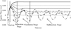 |
Fig. 12 Running process. |
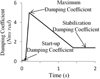 |
Fig. 13 Variable damping coefficient curve. |
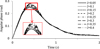 |
Fig. 14 Relationship between angular phase and rotational inertia with variable damping coefficient. |
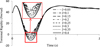 |
Fig. 15 Relationship between torsional rigidity and rotational inertia with variable damping coefficient. |
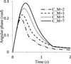 |
Fig. 16 Relationships between angular phase and different maximum damping coefficients. |
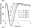 |
Fig. 17 Relationships between torsional rigidity and different maximum damping coefficients. |
3.5 Design of variable damping PMC
According to the above analysis, a suitable variable damping method was proposed to control the output speed stability of PMC. Figure 18 shows a novel variable damping PMC. It includes two parts: one is the traditional PMC, the other is a variable damping controller (VDC) which includes copper coil, iron core, round copper plate and controller.
The VDC is based on the electromagnetic damping effect principle. When copper plate rotates in the magnetic field, it will produce eddy current loss which causes eddy current resistance [22]. Eddy current resistance is proportional to the rotation speed of copper plate [23,24], so the eddy current resistance can be expressed as (30)
(30)
where B is the magnetic flux density of the magnetic field on the copper plate surface, ω is the angular velocity of the copper plate, a is a constant related with VDC structure.
In VDC, the magnetic field is created by a copper coil when the current flows through coil, and the magnetic flux density B is proportional to the current [25]. Because copper plate is very close to copper coil, it can be expressed as (31)
(31)
where µ is the permeability, N is the number of copper coil windings, L is the length of the copper coil, R is the radius of the copper coil and I is the current through the copper coil.
According to the equations (30) and (31), the eddy current resistance can be expressed as: (32)
(32)
where b is a constant related to the parameters of VDC.
So the damping coefficient Cv generated by VDC is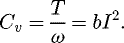 (33)
(33)
According to the equation (33), damping coefficient will change with the current, and it is how the VDC works. To verify the above analysis, a 3D finite element analysis (FEA) model of VDC is constructed and analyzed by ANSYS Maxwell, as shown in Figures 19 and 20, where copper plate radius and thickness are 200 mm, 3 mm, respectively; N is 1000; L is 50 mm; R is 50 mm and distance is 1 mm between copper plate surface and copper coil; the distance is 60 mm between the center of copper coil and copper plate.
In order to analyze the relationship between magnetic flux density B and the current I, the current was selected as variable. With the current increasing, the magnetic flux density increased rapidly as shown in Figure 21. The theoretical results of magnetic flux density were compared with the FEA results under various currents. Their results were very similar with each other and the relationship between magnetic flux density and the current showed a linear relation.
Then the relationship between eddy current resistance and angular velocity was analyzed. The angular velocity was selected as variable, and the magnetic flux density on copper plate surface was set as 1T. With the angular velocity increasing, the eddy current resistance increased rapidly, as shown in Figure 22. The results showed a linear relation between eddy current resistance and angular velocity, which was in good agreement with the equation (30).
VDC can realize the variable damping function by changing the current. Furthermore a suitable VDC can control the variation of the angular phase and produce an optimal torsional rigidity. This novel variable damping PMC can be applied to propulsor at a varying speed and improve the output speed stability. The presented method is suitable to not only PMC, but also other elastic transmission mechanisms.
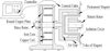 |
Fig. 18 Variable damping magnetic coupling. |
 |
Fig. 19 FEA model of VDCC. |
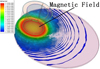 |
Fig. 20 FEA result of the magnetic field. |
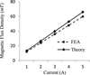 |
Fig. 21 Magnetic flux density changes with current. |
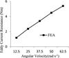 |
Fig. 22 Eddy current resistance changes with angular velocity. |
4 Conclusions
PMC is an important transmission mechanism used in propulsor, and its output speed stability is vital to propeller. The transmission system composed of PMC is a clutch system between the motor and propeller. In order to enhance PMC output speed stability, PMC dynamic equations were built based on Lagrange equation. In dynamic equations, the impact of installation and center-of-mass deviations on PMC dynamic characteristics were taken into account. According to the dynamic equations, angular phase between the master rotor and the slave rotor of PMC was calculated, which indicated PMC output speed stability. Then it was used as a major index to analyze and optimize PMC dynamic characteristics.
Damping coefficient, rotational inertia and torsional rigidity were selected as the variables to analyze the variation of the angular phase. The results showed that big damping coefficient was beneficial to PMC output speed stability while it would make a big stable value of the angular phase; small damping coefficient could make a small stable value while it would cause start-up oscillation which harmed PMC output speed stability. Rotational inertia had no effect on stable value of angular phase while it would affect start-up oscillation, and big torsional rigidity could make a small stable value of angular phase while it would cause start-up oscillation.
According to the impact of damping coefficient, rotational inertia and torsional rigidity on the angular phase, a variable damping method was proposed to control the output speed stability of PMC and reduce the start-up oscillation of angular phase. The angular phase varied smoothly and PMC performed better by this way. Finally, a novel variable damping PMC was designed, which was based on the electromagnetic damping effect principle. The theoretical calculation and FEA results confirmed that this design could be realized and applied to the propulsor to improve performance.
In the paper, a variable damping method that could be also applied to the control of other rotating machines was utilized to improve the performance of PMC. Then a variable damping controller that could be mounted on the rotating machine to improve its performance was designed to verify the feasibility of the method. This paper provides a reference for improving the output speed stability of the rotating machine by the means of variable damping.
Acknowledgments
The research is supported by 2018 National key research and development plan (Project no. 2018YFB2001300), the Fundamental Research Funds of Nanjing University of Aeronautics and Astronautics (Project no. 56YAH18100 and no. 90YAH18100), National Natural Science Foundation of China (Project no. 51775264) and National Key Laboratory of Science and Technology on Helicopter Transmission (Project no. HTL-A-19G06), which are gratefully acknowledged.
References
- V. Upadhyay et al., Design and motion control of Autonomous Underwater Vehicle, Amogh, in 2015 IEEE Underwater Technology (UT) (2015) 1–9 [Google Scholar]
- H.D. Nguyen, P. Niyomka, N. Bose, J. Binns, Performance evaluation of an underwater vehicle equipped with a collective and cyclic pitch propeller, IFAC Proc. 46, 167–172 (2013) [Google Scholar]
- T. Liu, Y. Hu, H. Xu, Z. Zhang, H. Li, Investigation of the vectored thruster AUVs based on 3SPS-S parallel manipulator, Appl. Ocean Res. 85, 151–161 (2019) [CrossRef] [Google Scholar]
- Z. Zhang, S. Cao, W. Shi et al., High pressure waterjet propulsion with thrust vector control system applied on underwater vehicles, Ocean Eng. 156, 456–467 (2018) [CrossRef] [Google Scholar]
- M. Eskandarian, P. Liu, A novel maneuverable propeller for improving maneuverability and propulsive performance of underwater vehicles, Appl. Ocean Res. 85, 53–64 (2019) [CrossRef] [Google Scholar]
- Z.Y. Ba Xin, L. Xiaohui, S. Zhaocun, A vectored water jet propulsion method for autonomous underwater vehicles, Ocean Eng. 74, 133–140 (2013) [CrossRef] [Google Scholar]
- S. McPhail, Autosub6000: A Deep Diving Long Range AUV, J. Bionic Eng. 6, 55–62 (2009) [Google Scholar]
- X. Zhou, Z. Liu, X. Meng, J. Liu, Influence of mechanical sealing surface shape of marine stern shaft on sealing performance, J. Traffic Transp. Eng. 16, 95–102 (2016) [Google Scholar]
- W. Litwin, Influence of main design parameters of ship propeller shaft water-lubricated bearings on their properties, Polish Marit. Res. 17, 39–45 (2010) [CrossRef] [Google Scholar]
- R.J.K. Wood, Marine wear and tribocorrosion, Wear 376, 893–910 (2017) [Google Scholar]
- J. Wu, Study on the leakage of Omega mechanical seal device, in Proceedings of the 2016 IEEE 11th Conference On Industrial Electronics And Applications (ICIEA) (2016) 276–278 [Google Scholar]
- C. Yang, Transmission characteristics of axial asynchronous permanent magnet couplings, J. Mech. Eng. 50, 76–84 (2014) [CrossRef] [Google Scholar]
- A.Y. Krasilnikov, Order of selection and design of magnetic clutches for sealed machines, Chem. Petrol. Eng. 49, 467–475 (2013) [CrossRef] [Google Scholar]
- A.Y. Krasilnikov, A.A. Krasilnikov, Magnetic clutches and magnetic systems in sealed machines, Chem. Petrol. Eng. 48, 306–310 (2012) [CrossRef] [Google Scholar]
- H.J. Shin, J.Y. Choi, S.M. Jang, Design and analysis of axial permanent magnet couplings based on 3D FEM, IEEE Trans. Magn. 49, 3985–3988 (2013) [Google Scholar]
- C. Lazaroff-Puck, Gearing up for Lagrangian dynamics, Arch. History Exact Sci. 69, 455–490 (2015) [CrossRef] [Google Scholar]
- H. Zhong, P. Du, F. Tang et al., Lagrangian dynamic large-eddy simulation of wind turbine near wakes combined with an actuator line method, Appl. Energy 144, 224–233 (2015) [Google Scholar]
- I. Goulos, V. Pachidis, P. Pilidis, Lagrangian formulation for the rapid estimation of helicopter rotor blade vibration characteristics, Aeronaut. J. 118, 861–901 (2014) [CrossRef] [Google Scholar]
- A. Niemenmaa, L. Salmia, A. Arkkio et al., Modeling motion, stiffness, and damping of a permanent-magnet shaft coupling, IEEE Trans. Magn. 46, 2763–2766 (2010) [Google Scholar]
- Y. Liu, C. Tong, J. Bai et al., Optimization of an 80 kW radial-radial flux compound-structure permanent-magnet synchronous machine used for HEVs, IEEE Trans. Magn. 47, 2399–2402 (2011) [Google Scholar]
- R. Ravaud, V. Lemarquand, G. Lemarquand, Analytical design of permanent magnet radial couplings, IEEE Trans. Magn. 46, 3860–3865 (2010) [Google Scholar]
- Z. Zhu, Z. Meng, 3D analysis of eddy current loss in the permanent magnet coupling, Rev. Sci. Instr. 87, 074701 (2016) [CrossRef] [Google Scholar]
- D. Zheng, D. Wang, S. Li et al., Eddy current loss calculation and thermal analysis of axial-flux permanent magnet couplers, AIP Adv. 7, 025117 (2017) [Google Scholar]
- B. Li, M. Li, Calculation and analysis of permanent magnet eddy current loss fault with magnet segmentation, Math. Probl. Eng. 2016, 1–6 (2016) [Google Scholar]
- N.R. Bouda, J. Pritchard, R.J. Weber et al., Methods of high current magnetic field generator for transcranial magnetic stimulation application, J. Appl. Phys. 117, 17 (2015) [Google Scholar]
Cite this article as: Z. Jian, L. Kun, Rotational speed control of magnetic coupling with variable damping method, Mechanics & Industry 21, 406 (2020)
All Tables
All Figures
|
Fig. 1 Permanent magnetic coupling. (a) The application of PMC; (b) angular phase in PMC. |
| In the text | |
|
Fig. 2 PMC structural parameters. |
| In the text | |
|
Fig. 3 PMC simplified model. |
| In the text | |
|
Fig. 4 Prototype. (a) Test rig: 1. DC Motor, 2. Torque-speed Sensor, 3. PMC, 4. Torque-speed Sensor, 5. Magnetic Powder Brake. (b) Schematic diagram of the test rig. |
| In the text | |
|
Fig. 5 Relationship between torque and angular phase. |
| In the text | |
|
Fig. 6 Relationship between torsional rigidity and angular phase. |
| In the text | |
|
Fig. 7 Relationship between angular phase and damping coefficient. |
| In the text | |
|
Fig. 8 Relationship between angular phase and damping coefficient with different rotational inertia. |
| In the text | |
|
Fig. 9 Relationship between angular phase and damping coefficient with different torsional rigidity. |
| In the text | |
|
Fig. 10 Relationships between angular phase and different rotational inertias. |
| In the text | |
|
Fig. 11 Relationships between angular phase and different torsional rigidities. |
| In the text | |
|
Fig. 12 Running process. |
| In the text | |
|
Fig. 13 Variable damping coefficient curve. |
| In the text | |
|
Fig. 14 Relationship between angular phase and rotational inertia with variable damping coefficient. |
| In the text | |
|
Fig. 15 Relationship between torsional rigidity and rotational inertia with variable damping coefficient. |
| In the text | |
|
Fig. 16 Relationships between angular phase and different maximum damping coefficients. |
| In the text | |
|
Fig. 17 Relationships between torsional rigidity and different maximum damping coefficients. |
| In the text | |
|
Fig. 18 Variable damping magnetic coupling. |
| In the text | |
|
Fig. 19 FEA model of VDCC. |
| In the text | |
|
Fig. 20 FEA result of the magnetic field. |
| In the text | |
|
Fig. 21 Magnetic flux density changes with current. |
| In the text | |
|
Fig. 22 Eddy current resistance changes with angular velocity. |
| In the text | |
Current usage metrics show cumulative count of Article Views (full-text article views including HTML views, PDF and ePub downloads, according to the available data) and Abstracts Views on Vision4Press platform.
Data correspond to usage on the plateform after 2015. The current usage metrics is available 48-96 hours after online publication and is updated daily on week days.
Initial download of the metrics may take a while.