| Issue |
Mechanics & Industry
Volume 22, 2021
|
|
|---|---|---|
| Article Number | 32 | |
| Number of page(s) | 17 | |
| DOI | https://doi.org/10.1051/meca/2021031 | |
| Published online | 30 April 2021 | |
Regular Article
Learning data-driven reduced elastic and inelastic models of spot-welded patches
1
ESI Group, Batiment Seville,
3 bis Saarinen,
50468,
Rungis, France
2
ESI Group Chair & PIMM Laboratory, Arts et Métiers Institute of Technology,
151 Boulevard de l’Hôpital,
75013
Paris, France
3
Renault,
1 Avenue du Golf,
78084
Guyancourt, France
4
Aragon Institute of Engineering Research, Universidad de Zaragoza,
Maria de Luna s/n,
50018
Zaragoza, Spain
* e-mail: This email address is being protected from spambots. You need JavaScript enabled to view it.
Received:
19
January
2021
Accepted:
8
April
2021
Abstract
Solving mechanical problems in large structures with rich localized behaviors remains a challenging issue despite the enormous advances in numerical procedures and computational performance. In particular, these localized behaviors need for extremely fine descriptions, and this has an associated impact in the number of degrees of freedom from one side, and the decrease of the time step employed in usual explicit time integrations, whose stability scales with the size of the smallest element involved in the mesh. In the present work we propose a data-driven technique for learning the rich behavior of a local patch and integrate it into a standard coarser description at the structure level. Thus, localized behaviors impact the global structural response without needing an explicit description of that fine scale behaviors.
Key words: Model Order Reduction / Spot-Welds / Machine Learning / Artificial Intelligence / Data-Driven Mechanics
© A. Reille et al., Published by EDP Sciences 2021
 This is an Open Access article distributed under the terms of the Creative Commons Attribution License (https://creativecommons.org/licenses/by/4.0), which permits unrestricted use, distribution, and reproduction in any medium, provided the original work is properly cited.
1 Introduction
High-fidelity simulations in computational structural mechanics involving large transformations (e.g., spot-weld rupture) become extremely expensive because of the strong nonlinearities, the extremely small time steps that usual explicit simulations imply and the extremely fine meshes required for describing adequately the different thermo-mechanical fields. These issues are not really new, having motivated in the past the proposal of a variety of homogenization procedures, today well experienced when the problems allow separating scales as well as identifying and extracting the so-called representative volume elements — RVE [1–5].
Moreover, many structures involve complex and rich space and time localized behaviors. This is the case when analyzing structures involving components joined by using spot welding, largely employed in car manufacturing. For avoiding high-resolution numerical analysis procedures, simplified models were proposed for addressing the spot-weld mechanical behavior into standard structural models, most of them based on the use of shell finite elements. These models usually consist of rigid or flexible beams, coincident nodes, ... enriched sometimes with some simplified structural elements within a patch in the shells that the spot-weld connects [6–17].
However, simplified modeling procedures can impact significantly the inelastic spot-weld behavior with the associated effects in the whole structure. Thus, for increasing accuracy, high-resolution 3D models are retained in many cases when addressing crash-test simulations. However, that accuracy increase is accompanied by an unreasonable computational effort. Even if the involved structural parts are in general modeled by using shell elements, when addressing spot-welds, their description needs the use of extremely fine 3D models able to represent the intrinsic themo-mechanical richness, involving elasticity, elasto-visco-plasticity, damage and fracture, as sketched in Figure 1. In addition, the fact of using very fine 3D discretizations (meshes) has another side effect, additionally to the natural increase of the number of degrees of freedom: the one associated with the reduction of the time step for keeping stable the usual explicit time integration.
Obviously, these difficulties do not represent real conceptual challenges. Models and solution procedures are mature and predictions are often in good agreement with the experimental results, despite the accuracy limits attained in the description of material behaviors in extreme loading conditions. The main issues concern neither the feasibility, nor the accessibility to the right material models, calibration procedures, computational algorithms, computing platforms and validation facilities, ... All these just referred topics attracted the interest of researchers and practicians during the last decades, and nowadays there is a solid, accurate and validated corpus of knowledge, with certified procedures and advanced analysis procedures [18]. For example, Renault recently announced a full car design with zero intermediate physical prototypes.
Definitively, the main difficulty concerns the computing time, a difficulty that persists despite the impressive advances around computer capability and the democratization of HPC. However, today the goal is not solving a problem to simulate a crash scenario, forinstance, but solving a number of them for different parameter choices (related to the loading but also to the structural parts, viz. materials, component thicknesses, ...). In other words: the so-called many-query framework. This is needed to optimize designs with respect to the selected quantities of interests (multi-objective optimization); to perform inverse analysis in order to calibrate component or global models, or to propagate the uncertainty that a certain deviation around a nominal parameter value will involve in the structural response [19].
For all the just mentioned problems, one should solve numerous scenarios while keeping all the richness in the description (high-fidelity simulations). Even if solving one case is acceptable regarding the computational cost, solving hundreds of them becomes unreasonable because of the excessive computational resources and processing time required. Model Order Reduction (intrusive and non-intrusive) seems an appealing route [20–23].
The present work proposes the construction of reduced models, by learning and assimilating the high-fidelity data coming from rich and expensive simulations performed offline, in order to represent the behavior of patches in which complex thermomechanical transformations occur. Thus, the whole structure accounts for the rich patch behavior, without the need of describing them explicitly. Their behavior manifest and express online in the structural response, without the necessity of simulating or co-simulating them.
The remaining part of the present paper is organized as follows:
-
Section 2 revisits the main concepts related to structural dynamics problems.
-
Section 3 discusses the possibility of describing the mechanical behavior introduced in Section 2 from the displacement and forces acting on the domain boundary.
-
Section 4 presents different methodologies for extracting such a condensed model from data (displacement and forces on the domain boundary) collected from high-fidelity solutions.
-
The learned models constructed in Section 4 on a patch are inserted in Section 5 into a larger structural system by using a local-global strategy.
-
Section 6 illustrates and discusses the local-global procedure in a simple case-study.
-
Section 7 addresses a complex inelastic behavior in a patch involving a spot-weld, and proves that its behavior can be learned by using the techniques described in Section 4, enabling fast and accurate enough predictions.
-
Section 8 groups the main conclusions and perspectives of the present work.
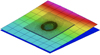 |
Fig. 1 Spot-weld 3D modeling. |
2 Structural solver
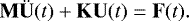
The general, semi-discretized form of the linear solid dynamics equations, writes
 (1)
(1)
where M, C and K are respectively the usual mass, damping and stiffness matrices. U represents the vector that contains the nodal displacements ( and
and  being respectively the associated accelerations and velocities) and F stands for the nodal external loads.
Sometimes damping vanishes, i.e., C = 0, but in the more general case it is usually assumed to be proportional, C = a0M + a1K, a fact that facilitates, among many other appealing advantages, the use of modal analysis, for forced responses (structural vibration). Thus, by ignoring (without loss of generality) the damping term, the previous semi-discrete form can be expressed as
 (2)
(2)
Explicit integration is preferred in fast dynamics involving strong nonlinearities, and for that the previous equation is expressed
 (3)
(3)
where Mℓ represent the lumped mass matrix that usually replaces the so-called consistent mass matrix M . The lumped mass matrix being diagonal, its inverse is trivial.
In the right-hand side of equation (3) we distinguish the internal and external force vectors, the former resulting from KU and the latter grouping all the external actions.
The explicit time discretization computes from the internal and external force vector at time t, Fint (t) and Fext (t) respectively, the associated acceleration  , from which the updated of velocities and displacements follow. Then, as soon as the displacement is known at time t + Δt, the associated internal forces must be evaluated Fint(t + Δt), before computing again the new acceleration, and so on.
If the domain Ω is partitioned with a mesh  composed of E subdomains ωe, e = 1, …, E, such that
  , with
  , the calculation of Fint needs the calculation of the stiffness of each subdomain ωe, Ke .
Remark 1.
-
In the previous expression the displacement and forces must be understood in their most general sense. When using shell elements for example, they involve general displacements (displacements and rotations) and their dual quantities, the generalized forces, consisting of forces and moments.
-
The subdomains ωe are in general the finite element partition of the domain Ω, but in fact it could also involve some patches or macro-patches as soon as a consistent approximation (ensuring the required continuity) is adopted to describe the displacement field.
-
To calculate the internal force vector, one could proceed to assemble first the elementary stiffness matrices Ke to construct K, from
![Mathematical equation: \[ {\mathbf{K}} = {{\mathsf{A}}}_{e=1}^((({{E}}))) \mathbf{K}^e, \]](/articles/meca/full_html/2021/01/mi210009/mi210009-eq10.png)
with A the assembling operator, and then compute Fint = KU(t); or compute the elementary internal force vectors
 and then assemble them into their global counterpart
  .
. -
When addressing inelastic behaviors, the stiffness matrix Ke, ∀e, is parametrized by a set of internal or latent variables grouped into the vector μ that allows condensing all the accumulated thermo-mechanical history experienced by each element, to express the present state without the necessity of explicitly considering all the experienced history. Thus, two approaches are possible: (i) the one that expresses the present state from all the experienced history and (ii) the one in which the present state depends on some latent variables expressed at the present time and that allows ignoring the past events whose actions or effects are condensed on those latent variables. Even if the last approach seems more frugal, many recurrent difficulties concern the nature, number, explainability, measurability and modeling of these latent variables.
3 On the condensed static and dynamic linear models
This section discusses condensed models in the elastic (static and dynamic) linear case [24] that, as proved, will depend on: (i) the existence of constant or time-dependent external forces acting inside the region concerned by the condensation procedure; and (ii) the necessity of considering the previous states that the time-integration of time-dependent models involve through their time derivatives.
3.1 Statics
The generic discrete form of mechanical problem involving elasto-statics in a given domain, can be expressed by
 (4)
(4)
that considering the variables on the domain boundary, UB, and the internal ones, UI, can written as
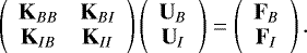 (5)
(5)
Developing the second relationship in equation (5)
 (6)
(6)
the first relationship in equation (5) results
 (7)
(7)
that can be rewritten as
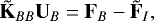 (8)
(8)
with  and
and  .
.
Remark 2.
-
If FI = 0 then
 , and fromequation (8) it follows that a direct relation between UB
and FB
exists.
, and fromequation (8) it follows that a direct relation between UB
and FB
exists. -
In the 1D case, UB and FB contains two components, i.e., both are defined in
 . If we apply
  and solve the associated static mechanical linear problem, the resulting FB
will represent the first column of
and solve the associated static mechanical linear problem, the resulting FB
will represent the first column of  . Then, the solution FB
related to UT = (0, 1) will give the second column of
. Then, the solution FB
related to UT = (0, 1) will give the second column of  .
. -
Still in 1D, if FI≠0, there are two internal variables, the two components of
 . Thus, independently of the intrinsic richness of FI, that is, of the number of internal nodes, all them express from only two variables, the two components of
 .
. -
Computing this two extra internal variables (again in a 1D setting) requires an extra calculation, for example if UB = 0, then
 .
.
3.2 Dynamical systems
This section analyses the effects of time derivatives following two alternative routes. The first operates from the discretized form and the second one employs a static condensation. The former will be illustrated in the next section by considering a linear model with first order derivatives, while the latter will be employed in the structural dynamics setting involving second order time derivatives.
3.2.1 Condensing discrete forms
If we consider the generic linear first order dynamical system
 (9)
(9)
the application of the standard Euler implicit time discretization reads
 (10)
(10)
with C′ = C∕Δt. By introducing the notation K = C′ + D and G = C′Un−1, the previousequation results
 (11)
(11)
that, with GB vanishing on the domain boundary where boundary conditions apply, the rationale employed in the previous section leads to
 (12)
(12)
where now, the two (in the 1D case) internal variables  are different at each time step because of the fact that
  depends on time, that is, on Un−1. This is indeed a bit perturbing, because the dependence of the condensed model on the previous time step solution seems difficult to implement practically.
3.2.2 Static condensation in elastodynamics
We considernow the elastodynamics problem
 (13)
(13)
and inspiredby relation (6), that relates internal degrees of freedom with the ones on the patch border in the static case,
![Mathematical equation: \[ {\mathbf{U}}_I = {\mathbf{K}}_{II}^{-1} {\mathbf{F}}_I - {\mathbf{K}}_{II}^{-1}{\mathbf{K}}_{IB} {\mathbf{U}}_B, \]](/articles/meca/full_html/2021/01/mi210009/mi210009-eq35.png)
one could consider [24]
 (14)
(14)
Remark 3. By using U = TUB in the static case, i.e.
![Mathematical equation: \[ {\mathbf{K}} {\mathbf{U}} = {\mathbf{F}} \rightarrow {\mathbf{K}} {\mathbf{T}} {\mathbf{U}}_B = {\mathbf{F}}, \]](/articles/meca/full_html/2021/01/mi210009/mi210009-eq37.png)
and premultiplying by TT,
![Mathematical equation: \[ {\mathbf{T}}^T {\mathbf{K}} {\mathbf{T}} {\mathbf{U}}_B = {\mathbf{T}}^T {\mathbf{F}}, \]](/articles/meca/full_html/2021/01/mi210009/mi210009-eq38.png)
we obtain the same solution that was already obtained in the static case.
By using the assumption expressed in equation (14), the dynamic problem reads
 (15)
(15)
that, in contrast with the previous procedure, only contains as internal variables the ones related to the external forces acting inside the considered patch. However, it does not depend on the internal solution at the previous time steps as was the case when discretizing first and then condensing.
However, in the just discussed procedure, its validity and accuracy strongly depend on the assumption (14), that is known to work quite well when dynamical (inertia) effects are moderate.
3.3 A new view inspired from Fourier analysis
By applying the Fourier transform (for the sake of simplicity, but without loss of generality, damping is here ignored or assumed proportional) to the displacement and forces  and
and  , the elastodynamics problem reads
 (16)
(16)
or
 (17)
(17)
This model is valid in forced regimes, because of the fact that when applying the Fourier transform, initial conditions (and with them, transient regimes) can not be enforced.
If for a while we assume that no external forces are applied within the domain, and that the dynamics involves a single frequency ω, by using the rationale followed in Section 3.1, a model relating  and
and  exists
 (18)
(18)
and it does not imply any internal variable.
Obviously to address a richer frequency spectrum, the superposition principle can be used. Thus, for any unitary loading applied at a boundary node and involving a single frequency, one could compute the associated response (displacement amplitude in all the nodes on the patch boundary). Thus, when a real load applies on the patch boundary, the Fourier transform applies at each node to extract the frequency content, and then the superposition principle is used to reconstruct the displacement amplitude at each node.
Now, byusing the Fourier inverse transform, the time evolution of the displacement at each node on the patch boundary results.
This route proves that in the forced elastodynamics regime, a model relating forces and displacements on the patch boundary exists and does not depend on any internal variable as soon as no external forces act inside the patch.
3.3.1 On the associate condensed model in the time-space
If starting from the single-frequency model (18), one comes back to the time domain, the following relation results
 (19)
(19)
where the indexes •f and •f refer to the fact that the model applies for the generic single frequency.
Obviously, linearity enables again using the superposition principle to address general loadings, and therefore concluding that again, in absence of external loads acting inside the patch, a relation between the forces and displacement on the patch border exists.
Even if the existence has been proved, its validity is restricted to forced dynamical regimes, and its numerical implementation remains quite tedious, because of the necessity to obtain many models and then combine them to address rich spectra. Another limitation of the just described procedure is its limitation to regions that do not contain resonances.
3.4 Learning condensed models
To avoid the difficulties just referred at the end of the previous section, the most direct procedure consists in assuming the general form
 (20)
(20)
or
 (21)
(21)
and learn the condensed models
 (22)
(22)
from the collected data UB and FB.
The learning procedure will be described in the next section. In the case in which external forces act within the patch, more data will be needed to learn the associated internal variables as indicated in Section 3.1.
Remark 4.
In the nonlinear case all the nonlinearities must be considered as effective forces acting inside the domain.
4 Model learning procedures
For the sake of simplicity, we start by assuming the discrete linear problem
 (23)
(23)
where F and U represent the input and output vectors respectively. In what follows forces and displacements at the nodes located on the patch boundary. Their respective size are N × 1 and N × 1.
As in the case of reduced order modeling (ROM), we assume that inputs and outputs are (to a certain degree of approximation) living in a sub-space of dimension n, much smaller than N. Thus, the rank of K is expected to be also n, even if a priori, it was ready to operate in a larger space of dimension N.
To learn the model K from the available data — displacement and force vectors —, two strategies were proposed in [25] within the so-called iDMD (incremental Dynamic Mode Decomposition), inspired from the original DMD [26].
4.1 Incremental Dynamic Mode Decomposition, iDMD
In what follows we describe the two constructors that will be considered in our numerical applications, the Rank-n and the progressive Rank-1 constructors.
4.1.1 Rank-n constructor
Here, we consider a set of S input-output couples (Fi, Ui), i = 1, …, S, and assume the model to be expressible from its low-rank form KLR
 (24)
(24)
where ⊗ denotes the tensor product, and Cj and Rj are the so-called column and row vectors. This expression is somehow similar to the separated representation used in the PGD (Proper Generalized Decomposition), the SVD (Singular Value Decomposition) or the CUR decomposition.
Let us define the functional  according to
 (25)
(25)
The choice of many different norms could be envisaged here. In what follows we consider the standard Frobenius norm ∥ • ∥F.
By considering matrices  and
and  containing in their columns vectors Fi and Ui respectively,the previous expression can be rewritten
 (26)
(26)
whose minimization results in KLR. A procedure based on the use of the PGD was proposed in [25].
In order to alleviate the computational issues related to the extremely high dimensional spaces N ≫ 1, a reduced counterpart can be defined, which proceeds by extracting a N-dimensional reduced basis from vectors Ui, grouped in the N × N matrix B . Thus, the displacement vectors can be expressed as Ui = Bui.
Now the discrete system (23) can be expressed in the reduced form
 (27)
(27)
or in its more compact counterpart
 (28)
(28)
Thus, from the available data, Ui and Fi, one first computes their reduced forms, ui = BTUi and fi = BTFi, and then the reduced model k from the previous rationale. It is important to note that, when considering the procedure based on the employement of the reduced basis B, filtering noisy data directly results from the consideration and construction of the reduced basis (high frequency modes are discarded inthe construction of reduced basis).
In the nonlinear case a tangent subspace can be found at each point of the data manifold. Consequently, the model, KLR works well in a neighborhood of the data U or F, i.e. KLR(U).
Thus, each time that a datum U arrives, the cluster to which it belongs, κ, is first identified. The cluster is identified from the distance between vector U and the U |κ related to each cluster (average of vectors U belonging to the cluster κ). Then, the low-rank model of that cluster,  , is chosen and the solution evaluated according to
 (29)
(29)
4.1.2 Progressive Rank-1 greedy construction
In this case we proceed progressively. We consider the first available datum, the pair (F1, U1). Thus, the first, rank-one reduced model reads
 (30)
(30)
When looking for a symmetric model the simplest choice consists of C1 = F1 and  , leading to
 (31)
(31)
Assume now that a second datum arrives, (F2, U2), from which we can also compute its associated rank-one approximation K2, and so on, for any new datum (Fi, Ui), that results in Ki, by simply replacing F1 and U1 by Fi and Ui respectively, in equation (31).
For any other U, the model could be interpolated from the just defined rank-one models, Ki, i = 1, …, S, according to
 (32)
(32)
with  the interpolation functions operating in the space of the data U, assumed decreasing with the distance between U and Ui.
This constructor seems particularly suitable in the nonlinear case. Thus, by defining the secant behavior at the middle point associated with F = 0.5(F1 + F2) as Ksec = 0.5(K2 −K1), we will have K = K1 + Ksec = 0.5(K1 + K2), fact that allows viewing the progressive greedy construction and its associated interpolation as a linearization procedure.
4.2 Learning parametric models
Again within the PGD rationale, all the previous discussion and developments can be extended to parametric settings. Thus, linear and nonlinear models (using the rank-N or the greedy constructors previously presented) are associated to particular values of the model parameters grouped into the vector μ : μ1, ⋯, μP. Thus, as soon as models K(μp), p = 1, …, P, are available, the one related to μ, is computedfrom
 (33)
(33)
with  the interpolation functions operating in the parametric space, assumed to be decreasing with the distance between μp and μ.
When addressing highly multidimensional models  , with M ≫ 1, usual interpolations fail. Thus, the sPGD [23] interpolation making use of the separated representations at the heart of the PGD can be applied.
4.3 Learning stable models
When the time evolution of the state z (the state here groups displacement and velocities) of a system is approached in a discrete manner, two stability concepts become key players: (i) the one related to the model itself (in general models describing physics are stable — their time evolution do not diverge—but when these models are learned from data stability can be lost) and (ii) the one associated with time discretization strategy. Both are implicit in the discrete form
 (34)
(34)
where the index •n, n ≥1, refers to the time instant tn = nΔt. If M is symmetric, it can be diagonalized, leading to the orthonormal basis V that enablesexpressing the state as
 (35)
(35)
and with VTMV = Λ (Λ being the diagonal matrix containing all the eigenvalues), equation (34) reads
 (36)
(36)
or by recurrence
 (37)
(37)
To have a solution when n →∞, i.e. t →∞, the greater eigenvalue needs to be lower than one, i.e., ρ(M) ≤ 1 (with ρ(M) the spectral radius of matrix M).
Thus, if S phase states (grouping displacement and velocity) are available for a given parameter μ, and we organize them in the columns of matrices Z and  , with
  and
and  , the calculation of a stable model M consists of looking for minimizing the Frobenius norm
  , where the procedures described in Section 4.1.1 can be applied (including the reduced formulation) while enforcing the stability condition ρ(M) ≤ 1.
5 Global-Local structural solver
The procedure that we propose considers the patch domain ω immersed into the whole domain Ω as sketched in Figure 2. The patch ω is equipped with a 3D fine discretization surrounded by a transition zone equipped with a 2D representation (e.g., by using shell elements) to better connect with the remaining part of the structure  where a fully 2D model applies. Domains ω and
  are sketchedin Figure 3
 |
Fig. 2 2D/3D patch ω immersed into the whole domain Ω. |
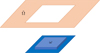 |
Fig. 3 Patch ω
and the remaining structure |

5.1 Patch modelling
Now, the isolated patch ω is subjectedto a very large variety of loadings applied on its boundary ∂ω, by enforcing the time evolution of the displacement in the different nodes on ∂ω, which result in vectors Ui(t), i = 1, …, S, with  , where the dimension
  scales with the number of nodes on thepatch boundary ∂ω multiplied by the number of degrees of freedom per node.
By solving the S quasi-static inelastic problems in ω, one obtainsthe displacement at each node in the fine patch mesh,  , as well as the forces on ∂ω that constitute vectors Fi(t).
Now, the data pairs (Ui, Fi), i = 1, …, S, at any time, should suffice to define thelocal rank-n or rank-one models according to the procedures described in Section 4.
In whatfollows the following assumptions are made: (i) no external forces apply inside the patch ω; (ii) the mechanical effects are very important compared to the ones related to the dynamical effects (inertia) enabling static condensation in reference to the discussion in Section 3 (this assumption seems quite reasonable except close to the rupture stage); and (iii) irreversible transformations (plasticity, damage and fracture) must be parametrized from the introduction of some latent variables grouped into the vector μ, that with the loading quite monotonic in practice (as inferred from the analysis of crash simulations), can be associated to the displacement on the boundary itself.
5.2 Time integration
By assuming the patch stiffness Kω(μ) known, the time integration performs at time t as sketched in Figure 4, by chaining the following calculations:
-
From the nodal displacements in
 ,
,
 , the ones acting on the patch boundary U(t) are extracted.
 -
From U(t) and the present internal state μ(t) the patch database is interrogated to recover the patch model Kω(μ(t)).
-
Evaluate the forces on the patch boundary F(t) = Kω(μ(t))U(t);
-
Compute the nodal accelerations in
 by solving the momentum balance:
 (38)
(38)
where  refers to quantities defined in
  whereas F(t) traduces thepatch effects;
-
Integrate acceleration to compute velocities and displacements at time t + Δt.
-
Update the latent variables μ(t + Δt).
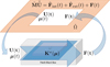 |
Fig. 4 Time integrator making use of the learned patch model. |
6 Global-local procedure validation
In the present section we will consider a simple problem to illustrate all the just discussed concepts and also to validate the whole methodology. For the sake of simplicity in the exposition, we consider the 3D model shown in Figure 5, where the domain Ω is composed of a patch ω (employed as a breaking fusible) where inelastic deformation is expected to localize during the loading, and the remaining part  where only elastic deformations will occur.
Even if Figure 5 represents the mechanical system, the computational domain Ω considered in the present analysis was shortened, in particular the domain exhibiting an elastic behavior  , in order to not increase unnecessarily the computational efforts related to the fully 3D finite element discretization. Figure 6 presents the computational model Ω, and its partition into the patch ω and the elastic region
  .
.
In the present case, the global-local solution procedure sketched in Figure 4, reduces to the one shown in Figure 7. The elastic behavior is defined by the elastic modulus E = 6.68 N/m2, the Poisson coefficient ν = 0.35 and the material density ρ = 2700 Kg/m3. The elastoplastic behavior is described from the Krupkowski model with isotropic hardening, whose yield stress σY reads
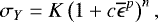 (39)
(39)
with K = 0.285 109 N/m2, c = 125 and n =0.1.
The dimensions of the computational domain shown in Figure 6 are Hx = 350 mm, Hy = 80 mm and Hz = 20 mm, with the patch ω having  mm.
mm.
To validate the global-local solution procedure, we first consider a purely elastic behavior, and then a loading inducing elastoplasticdeformations at the patch level.
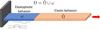 |
Fig. 5 3D model Ω
composed of a patch ω
where inelastic deformation is expected localizing during the loading and the remaining part
|

 |
Fig. 6 Computational domain Ω
(left) and its partition |

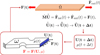 |
Fig. 7 Global-local time integration. |
6.1 Linear behavior
In this first case study the loading induces stresses that remain always and everywhere below the yield stress. In what follows we first present the results obtained from a fully 3D discretization of the whole domain Ω that will serve as reference solution. Then, the patch elastic behavior will be learned and finally used within the global-local integration procedure previously described.
6.1.1 Fully 3D finite element discretization
Figure 8 shows the applied load on the right boundary of the whole structure depicted in Figure 6. Figure 9 presents the quasi-static time evolution of the x-component of the displacement, averaged on the right surface of the specimen (the one on which traction applies and that presents an almost uniform displacement along the x-direction),  , defined from
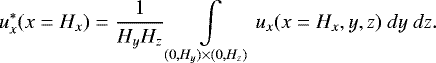 (40)
(40)
Figure 10 compares the displacement  solutions obtained by using an undamped and damped elasto-dynamic explicit integration, where the effects of the dynamics can be noticed, mainly in the undamped case. The damped solution remains close to the reference solution depicted in Figure 9. To facilitate the solutions comparison Figure 11 shows the reference solution (quasi-static) and the explicit damped one.
The final (at t = 3 × 10⁻³ s) 3D displacement field obtained with the explicit damped integration is shown in Figure 12, that remains in perfect agreement with the one obtained by using a quasi-static integration.
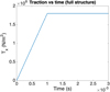 |
Fig. 8 Applied traction on the right boundary of the whole structure, along the x-direction. |
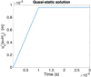 |
Fig. 9 Averaged displacement of the structure right surface: |

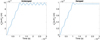 |
Fig. 10 Averaged displacement of the structure right surface: |

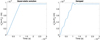 |
Fig. 11 Quasi-static (left) versus explicit damped (right) solutions. |
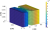 |
Fig. 12 Displacement field ux obtained at time t = 3 × 10⁻³ s. |
6.1.2 Extracting the patch elastic model
In the purely elastic case and being only interested in the relation between the applied traction and the induced displacements along the x-direction at the patch surface  (that remains almost uniform in the whole surface) a single loading, as the one depicted in Figure 13 consisting of the traction Tx (t), suffices to extract the reduced behavior (reduced in the sense discussed in [25] and in Section 4) shown in Figure 14 relating the x-components of the applied force Fx and the induced displacement Ux.
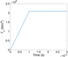 |
Fig. 13 Applied traction along the x-direction on the patch surface |

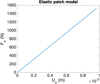 |
Fig. 14 Applied force versus induced displacement on the patch surface |

6.1.3 Global-local integration
Now, once the patch behavior has been extracted, one could be interested in solving the quasi-static elastodynamics problem in  while using the patch model just extracted, by employing the global-local integration previously described and illustrated in Figure 7.
Now, the structural loading shown in Figure 8 will be applied on the right surface of  , x = Hx, while on itsleft boundary the patch model is applied. The displacement on x = Hx obtained by using an explicit damped integration is compared with the reference one (given in Fig. 9) in Figure 15, proving the ability of the proposed global-local integration to reproduce the mechanical response.
Figure 16 compares both damped explicit integration, the one related to the solution in the whole domain and already depicted in Figure 11 (right) and the one related to the global-local integration just depicted in Figure 15 (right). Even if both solutions are very similar, it seems that the one obtained by using the global-local integration, that is, the one making use of the patch model, increases the frequency of the spurious oscillations generated by the dynamical effects.
To better analyze these effects, Figure 17 compares now the undamped solutions, the one related to the solution in the whole domain and already depicted in Figure 11 (left) and the one related to the global-local integration. The last figure clearly proves that the use of the static patch model affects the dynamics because it reflects the waves.
To perform better in dynamics special care must be paid in constructing a patch model able to perform in the dynamical regime as discussed in Section 3. However, in practical applications in which patches are very localized in large structures (e.g. spot-welds in car structures) patch static models have a minor effect on the global dynamical response.
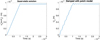 |
Fig. 15 Quasi-static solution given in Figure 9 (left) versus the explicit damped obtained using the global-local integration schema (right). |
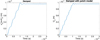 |
Fig. 16 Damped explicit integrations: (left) the one related to the solution in the whole domain and already depicted in Figure 11 (right); (right) the one related to the global-local integration just depicted in Figure 15 (right). |
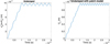 |
Fig. 17 Undamped explicit integrations: (left) the one related to the solution in the whole domain and already depicted in Figure 10 (right) and (right) the one related to the global-local integration. |
6.2 Inelastic behavior
In this second case study the loading induces stresses above the yield stress in the region of ω with smaller cross section.
In whatfollows we first present the results obtained from a fully 3D discretization of the whole domain Ω that will serve asreference solution. Then, the patch inelastic behavior will be learned and finally used within the global-local integration procedure previously described.
6.2.1 Fully 3D finite element discretization
The applied load is again the one shown in Figure 8. Figure 18 presents the quasi-static time evolution of the x-component of the displacement, averaged on the right surface of the specimen (the one on which traction applies and that present an almost uniform displacement along the x-direction), i.e.  previously defined in equation (40).
Figure 19 shows the displacement  obtained by using a damped elasto-dynamic explicit integration, where again the effects of the dynamics can be noticed. The damped solution remains reasonably close to the reference solution depicted in Figure 18. To facilitate the solution comparison, Figure 20 shows the reference solution (quasi-static) and the explicit damped one. The final (t =3 × 10⁻³ s) plastic localization is shown in Figure 21.
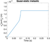 |
Fig. 18 Displacement of the structure right surface: |

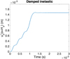 |
Fig. 19 Displacement of the structure right surface: |

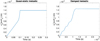 |
Fig. 20 Quasi-static (left) versus explicit damped (right) in the inelastic case. |
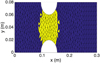 |
Fig. 21 Plastic localization at time t = 3 × 10⁻³ s (elements colored in yellow are experiencing plastic deformation). |
6.2.2 Extracting the patch inelastic model
Being only interested in the relation between the applied traction and the induced displacements along the x-direction at the patch surface  (that is almost uniform on the surface) in monotonous loadings, a single loading, the one depicted in Figure 13 consisting of the traction Tx(t), suffices to extract the reduced behavior, shown in Figure 22 relating the x-components of the applied force Fx and the induced displacement Ux.
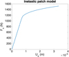 |
Fig. 22 Applied force versus induced displacement on the patch surface |

6.2.3 Global-local integration
Once the patch behavior has been extracted, we are solving the quasi-static elastodynamics problem in  while using the patch model just extracted, by employing the global-local integration previously described and illustrated in Figure 7.
Now, the structural loading shown in Figure 8 will be applied on the right surface of  , x = Hx, while in its left boundary the patch model is applied. The displacement on x = Hx obtained by using an explicit damped integration is compared with the reference one (given in Fig. 18) in Figure 23, proving the ability of the proposed global-local integration to reproduce the mechanical response.
Figure 24 compares both damped explicit integrations, the one related to the solution in the whole domain depicted in Figure 20 (right) and the one related to the global-local integration just depicted in Figure 23 (right). Even if both solutions are very similar, it seems that the one obtained by using the global-local integration, that is, the one making use of the patch model, increases the frequency of the spurious oscillations generated by the dynamical effects, already discussed previously.
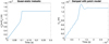 |
Fig. 23 Quasi-static solution given in Figure 18 (left) versus the explicit damped obtained using the global-local integration (right). |
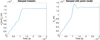 |
Fig. 24 Damped explicit integrations: (left) the one related to the solution in the whole domain and already depicted in Figure 20 (right); (right) the one related to the global-local integration just depicted in Figure 23 (right). |
7 Learning the spot-weld model
This section addresses a patch inelastic behavior, and model it from the collected data by using the techniques previously introduced, discussed and illustrated, in particular the progressive rank-1 constructor. In the present case, the local-global strategy is not employed, constituting a work in progress for addressing valuable industrial applications.
We consider the spot-weld depicted in Figure 25 with two different loading typologies, the one corresponding to the left and the one to the right. The upper images depict the displacement degrees of freedom that were frozen while applying the displacements as depicted by the red arrows in the images at the bottom, by prescribing different velocity values.
For the different loading cases, a complete design of experiments –DoE– was considered, with the minimum and maximum values, 0 and 0.1 m/s respectively, of the velocities applied on the domain boundary in each coordinate direction. The resulting 3D problems were simulated and the forces at the 24 nodes located on the boundaries of each of the two plates extracted atdifferent instant (with about 25000 time steps in each simulation), from the beginning of the loading until the spot-weld totally breaks. By excluding from the DoE the trivial cases with null applied velocities, the 25 = 32 experiments (2 loading typologies and two velocities along each of the three coordinate direction) reduces to 28 numerical experiments.
Form all these simulations, 70.000 displacement-force couples were extracted, leading to the same number of stiffness matrices that composed the mechanical dictionary.
Then, 6 test-cases were defined for validating the calculation procedure, with the loading and magnitude of the applied velocities reported in Table 1. Figure 26 compares the associated high-fidelity solutions (reference solutions) and the ones predicted by using the dictionary.
The agreement is globally acceptable, taking into account the low number of available data (size of the training set). The relative errors remains lower than 10% before the fracture starts, reaching maximum relative errors of 20% in the final steps. It is important to note that the parametric loading space is extremely rich and intensive simulation should be required to populate adequately the space in order to improve robustness, and to address general complex loadings.
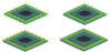 |
Fig. 25 Spot-weld supporting conditions (green arrows in the figures at the top) and enforced displacements (red arrows in the figures at the bottom) for two different loading typologies: left and right images. |
Validation test-cases.
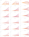 |
Fig. 26 Predicted forces for the loadings belonging to the test set (images at each row refers to a different loading condition): (left) Fx; (center) Fy; and (right) Fz. |
8 Conclusions
This paper proposes an integrated methodology able to learn reduced models to be employed in efficient computational inelasticity.
In particular, when they are applied to model rich and localized behaviors within a patch, the simulation of the whole structure can be performed by keeping the patch effects but without needing to resolve it.
The main advantages of such a procedure are, first the reduction in the number of degrees of freedom (patches usually imply fine 3D discretization). Second, the increase of the time step in explicit integrations, because now the integration stability is not governed anymore by the size of the smallest element (the ones needed for describing the solution at the patches level in standard simulation).
We illustrate the existence of condensed models, then the possibility of using them in a local-global integration and finally, the possibility of extracting accurate enough models of spot-welds.
It is still too early to conclude on both the accuracy and the performances of the proposed methodology when applied to industrial problems of relevance. The present paper presented a methodology for learning inelastic mechanical models, illustrated the local-global performances in a quite simple case-study, and succeeded to establish the model of a patch involving a spot-weld. However, in order to conclude on its industrial applicability, the model should be enriched: (i) by enlarging the sampling used in the model training; and (ii) by setting-up the local-global methodology with a fine study of the error propagation and the CPU time savings. The performances are expected significant because of the high number of spot-welds (thousands in a car structure) and the ultra-fast evaluation of the constructed patch model.
Acknowledgements
Authors acknowledge the contributions of Dr. Giacomo Quaranta concerning the verification of the global-local modeling framework.
References
- R. de Borst, Challenges in computational materials science: multiple scales, multi-physics and evolving discontinuities, Comput. Mater. Sci. 43, 1–15 (2008) [Google Scholar]
- F. Feyel, Multiscale FE2 elastoviscoplastic analysis of composite structures, Comput. Mater. Sci. 16, 344–354 (1999) [CrossRef] [Google Scholar]
- H. Lamari, A. Ammar, P. Cartraud, G. Legrain, F. Jacquemin, F. Chinesta, Routes for efficient computational homogenization of non-linear materials using the Proper Generalized Decomposition, Arch. Comput. Methods Eng. 17, 373–9 (2010) [Google Scholar]
- J. Yvonnet, D. Gonzalez, Q.-C. He, Numerically explicit potentials for the homogenization of nonlinear elastic heterogeneous materials, Comput. Methods Appl. Mech. Eng. 198, 2723–2737 (2009) [Google Scholar]
- M.G.D. Geers, V.G. Kouznetsova, W.A.M. Brekelmans, Multi-scale computational homogenization: trends and challenges. J. Comput. Appl. Math. in press, DOI: 10.1016/j.cam.2009.08.077 [Google Scholar]
- J. Backhans, A. Cedas, A finite element model of spot welds between non-congruent shell meshes Ñcalculation of stresses for fatigue life prediction. MSc thesis, Analysis report, 93841-2000-106, Volvo Car Corporation, Gothenburg, Sweden, 2000 [Google Scholar]
- W. Chen, X. Deng, Performance of shell elements in modelling spot-welded joints, Finite Elem. Anal. Des. 35, 41–57 (2000) [Google Scholar]
- H. Di Fant-Jaeckels, A. Galtier, Fatigue life prediction model for spot welded structures, in Fatiguedesign 1998 symp, vol. I. Espoo (Finland), May 1998 [Google Scholar]
- J. Fang, C. Hoff, B. Holman, F. Mueller, D. Wallerstein, Weld modelling with MSC. Nastran. In: 2nd MSC worldwide automotive user conf, Dearborn, MI, 2000 [Google Scholar]
- D. Heiserer, M. Charging, J. Sielaft, High performance, process oriented, weld spot approach, in 1st MSC worldwide automotive user conf, Munich, Germany, September 1999 [Google Scholar]
- K. Pal, D.L. Cronin, Static and dynamic characteristics of spot welded sheet metal beams, J. Eng. Ind. Trans ASME 117, 316–322 (1995) [Google Scholar]
- A. Rupp, K. Storzel, V. Grubisic, Computer aided dimensioning of spot-welded automotive structures, in SAE technical paper 950711, Int congress and exposition, Detroit (USA), 1995 [Google Scholar]
- P. Salvini, F. Vivio, V. Vullo, A spot weld finite element for structural modelling, Int. J. Fatigue 22, 645–56 (2000) [Google Scholar]
- F. Vivio, G. Ferrari, P. Salvini, V. Vullo, Enforcing of an analytical solution of spot welds into finite elements analysis for fatigue life estimation, Int. J. Comput. Appl. Technol. 15, 218–229 (2002) [Google Scholar]
- Y. Zhang, D. Taylor, Fatigue life prediction of spot welded components, in Proc of the seventh int fatigue conf, 8-12 June 1999, Beijing [Google Scholar]
- Y. Zhang, D. Taylor, Optimisation of spot-welded structures, Fin. Elem. Anal. Des. 37, 1013–1022 (2001) [Google Scholar]
- S. Zhang, Recovery of notch stress and stress intensity factors in finite element modelling of spot welds, in Proc. of Nafems world congress 99, Newport (USA), April 1999 [Google Scholar]
- H. Li, C.A. Duarte, A two-scale generalized finite element method for parallel simulations of spot welds in large structures, Comput. Methods Appl. Mech. Eng. 337, 28–65 (2018) [Google Scholar]
- V. Limousin, X. Delgerie, E. Leroy, R. Ibanez, C. Argerich, F. Daim, J.L. Duval, F. Chinesta, Advanced model order reduction and artificial intelligence techniques empowering advanced structural mechanics simulations, Application to crash test analyses. Mech. Ind. 20, 804 (2019) [Google Scholar]
- D. Borzacchiello, J.V. Aguado, F. Chinesta, Non-intrusive sparse subspace learning for parametrized problems, Arch. Comput. Methods Eng. 26, 303–326 (2019) [Google Scholar]
- F. Chinesta, A. Leygue, F. Bordeu, J.V. Aguado, E. Cueto, D. Gonzalez, I. Alfaro, A. Ammar, A. Huerta, Parametric PGD based computational vademecum for efficient design, optimization and control, Arch. Comput. Methods Eng. 20, 31–59 (2013) [Google Scholar]
- F. Chinesta, A. Huerta, G. Rozza, K. Willcox, Model Order Reduction. Chapter in the Encyclopedia of Computational Mechanics, Second Edition, E. Stein, R. de Borst & T. Hughes Edts, John Wiley & Sons, Ltd. (2015) [Google Scholar]
- R. Ibanez, E. Abisset-Chavanne, A. Ammar, D. Gonzalez, E. Cueto, A. Huerta, J.L. Duval, F. Chinesta, A multi-dimensional data-driven sparse identification technique: the sparse Proper Generalized Decomposition. Complexity 2018, Article ID 5608286 (2018) [Google Scholar]
- J.Garcia-Martinez, F.J. Herrada, L.K.H. Hermanns, A. Fraile, F.J. Montans, Parametric studies in computational dynamics: Selective modal re-orthogonalization versus model order reduction methods, Adv. Eng. Softw. 108, 24–36 (2017) [Google Scholar]
- A. Reille, N. Hascoet, C. Ghnatios, A. Ammar, E. Cueto, J.L. Duval, F. Chinesta, R. Keunings, Incremental dynamic mode decomposition: a reduced-model learner operating at the low-data limit, C. R. Mecanique 347, 780–792 (2019) [Google Scholar]
- P.J. Schmid, Dynamic mode decomposition of numerical and experimental data, J. Fluid Mech. 656, 5–28 (2010) [Google Scholar]
Cite this article as: A. Reille, V. Champaney, F. Daim, Y. Tourbier, N. Hascoet, D. Gonzalez, E. Cueto, J.L. Duval, F. Chinesta, Learning data-driven reduced elastic and inelastic models of spot-welded patches. Mechanics & Industry 22, 32 (2021)
All Tables
All Figures
|
Fig. 1 Spot-weld 3D modeling. |
| In the text | |
|
Fig. 2 2D/3D patch ω immersed into the whole domain Ω. |
| In the text | |
|
Fig. 3 Patch ω
and the remaining structure |
| In the text | |
|
Fig. 4 Time integrator making use of the learned patch model. |
| In the text | |
|
Fig. 5 3D model Ω
composed of a patch ω
where inelastic deformation is expected localizing during the loading and the remaining part
|
| In the text | |
|
Fig. 6 Computational domain Ω
(left) and its partition |
| In the text | |
|
Fig. 7 Global-local time integration. |
| In the text | |
|
Fig. 8 Applied traction on the right boundary of the whole structure, along the x-direction. |
| In the text | |
|
Fig. 9 Averaged displacement of the structure right surface: |
| In the text | |
|
Fig. 10 Averaged displacement of the structure right surface: |
| In the text | |
|
Fig. 11 Quasi-static (left) versus explicit damped (right) solutions. |
| In the text | |
|
Fig. 12 Displacement field ux obtained at time t = 3 × 10⁻³ s. |
| In the text | |
|
Fig. 13 Applied traction along the x-direction on the patch surface |
| In the text | |
|
Fig. 14 Applied force versus induced displacement on the patch surface |
| In the text | |
|
Fig. 15 Quasi-static solution given in Figure 9 (left) versus the explicit damped obtained using the global-local integration schema (right). |
| In the text | |
|
Fig. 16 Damped explicit integrations: (left) the one related to the solution in the whole domain and already depicted in Figure 11 (right); (right) the one related to the global-local integration just depicted in Figure 15 (right). |
| In the text | |
|
Fig. 17 Undamped explicit integrations: (left) the one related to the solution in the whole domain and already depicted in Figure 10 (right) and (right) the one related to the global-local integration. |
| In the text | |
|
Fig. 18 Displacement of the structure right surface: |
| In the text | |
|
Fig. 19 Displacement of the structure right surface: |
| In the text | |
|
Fig. 20 Quasi-static (left) versus explicit damped (right) in the inelastic case. |
| In the text | |
|
Fig. 21 Plastic localization at time t = 3 × 10⁻³ s (elements colored in yellow are experiencing plastic deformation). |
| In the text | |
|
Fig. 22 Applied force versus induced displacement on the patch surface |
| In the text | |
|
Fig. 23 Quasi-static solution given in Figure 18 (left) versus the explicit damped obtained using the global-local integration (right). |
| In the text | |
|
Fig. 24 Damped explicit integrations: (left) the one related to the solution in the whole domain and already depicted in Figure 20 (right); (right) the one related to the global-local integration just depicted in Figure 23 (right). |
| In the text | |
|
Fig. 25 Spot-weld supporting conditions (green arrows in the figures at the top) and enforced displacements (red arrows in the figures at the bottom) for two different loading typologies: left and right images. |
| In the text | |
|
Fig. 26 Predicted forces for the loadings belonging to the test set (images at each row refers to a different loading condition): (left) Fx; (center) Fy; and (right) Fz. |
| In the text | |
Current usage metrics show cumulative count of Article Views (full-text article views including HTML views, PDF and ePub downloads, according to the available data) and Abstracts Views on Vision4Press platform.
Data correspond to usage on the plateform after 2015. The current usage metrics is available 48-96 hours after online publication and is updated daily on week days.
Initial download of the metrics may take a while.