| Issue |
Mechanics & Industry
Volume 18, Number 4, 2017
|
|
|---|---|---|
| Article Number | 406 | |
| Number of page(s) | 6 | |
| DOI | https://doi.org/10.1051/meca/2017011 | |
| Published online | 28 August 2017 | |
Regular Article
A computational fluid dynamics (CFD) approach for the modeling of flux in a polymeric membrane using finite volume method
School of Chemical and Materials Engineering, National University of Sciences and Technology (NUST),
Islamabad, Pakistan
* e-mail: This email address is being protected from spambots. You need JavaScript enabled to view it.
Received:
2
June
2015
Accepted:
10
February
2017
Abstract
The computational fluid dynamics (CFD) modeling in this study observes steady-state mass transfer in a polymeric membrane. The efficiency, robustness, and reliability of recent numerical methods for finding solutions to flow problems have given rise to the implementation of CFD as a broadly used analysis method for engineering problems like membrane separation system. This study is novel due to the implementation of user-defined scalar diffusion equation by using user-defined functions in finite volume method (FVM). During the implementation of governing equation and boundary conditions important details of the FVM are discussed in detail. In this research, the flux profile is reported calculated from the pressure gradient for a steady-state problem.
Key words: computational fluid dynamics / finite volume method / mass transfer / user-defined functions / polymeric membrane
© AFM, EDP Sciences 2017
1 Introduction
Computational methods have the ability for improving the understanding of flow problems in membrane separation systems. They have the proficiency of giving data on flow conditions at any point of the geometry without troubling the flow. Furthermore, the implementation of mathematical modeling expressively decreases the costs, risks, and time related to performing repetitive experiments. One numerical method implemented for simulating fluid flow is known as computational fluid dynamics (CFD) [1–5]. CFD has become a more commonly implemented method in the research area of membrane science [6–8], with several researchers using this tool to obtain understanding into the phenomena taking place inside membrane modules, to support the design process and increase the performance of modules. Also, flow data can explain at any point and time throughout the simulation. The assessment of these flow variables is conceivable, deprived of any trouble to the primary flow. As an analysis method, CFD gives the permission to change fluid properties, operating conditions, and geometric characteristics of the flow channels in a flexible but defined way [9]. The geometric parameters of the channels change, deprived of the requirement to make and check new meshes. It signifies a major benefit of the CFD tool over traditional experimental methods [10]. Because of its easiness and minor computational necessities, several scholars have selected CFD for modeling membrane in two and three dimensions, as is presented by the size of effort achieve in this field [11–16]. Therefore, CFD considers as a consistent technique, and progressively unsteady flow and studies are developing, mostly finding decent similarity within calculated and experimental results [17–19].
Organic and inorganic materials are used to synthesize membranes for gas separation. In late 1970s commercial polymeric membranes, i.e. polydimethylsiloxane, cellulose acetate, polyether sulphone, etc. for gas applications became available [20]. Membranes based on polymers establish extensive use in the separation of N2, O2, and CO2, however at lower temperatures because of low thermostability of polymeric materials, though several engineering methods include the production of gasses at high temperatures. One case is the production of syngas (a mixture of carbon dioxide and hydrogen) through coal gasification or natural gas reforming [21]. Preliminary research directed to differing ideas on the consequence of gas polarization, which is a link with the reduction of the additional permeable gas through the membrane. This effect allows for the increase of the less permeable gas on the feed side and tends to increase in significance for membranes providing very high selectivities [22]. High feed flow rate decreases the concentration polarization in a membrane module [23].
Membrane gas system is an important separation process of chemical engineering. In this research, the research was a focus on mass transfer through the domain of a 2D rectangular membrane using general scalar diffusion equation with mixed boundary conditions (BCs). This study covers the solution of the steady-state problem with the formulation of BCs for first-order discretization technique. The UDF integrates with finite volume method (FVM) based CFD solver (ANSYS FLUENT™) for the solution. The contours of rectangular membrane domain show the behavior of flux through a polymeric membrane. The mass transfer problem of flow in a membrane is a less focused area, especially for high-pressure gradient due to its complexity. This study is an effort to solve user-defined scalar (UDS) diffusion equation to solve complex diffusion phenomena in a membrane.
2 CFD modeling
The mass transfer modeling and the aspects of transport mechanisms permanently linked with the fundamental properties of the material used to synthesize a membrane. A universal principle of membrane operation is that there must be a driving force for a gas molecule to diffuse from the feed domain to the permeate side. This driving force is expressed as a pressure gradient in the case of mass transfer in polymer-based membranes. The membrane describes as a zero-thickness wall. The overall mass balance is written as:
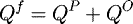 (1)
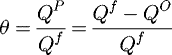
Qf is the feed flow rate, QO is residue flow rate, and QP is the permeate flow rate. The overall component balance is written as:
(1)
Qf is the feed flow rate, QO is residue flow rate, and QP is the permeate flow rate. The overall component balance is written as:
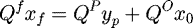 (2)xf, x0 and y0 are feed mole fraction, retentate mole fraction and permeate mole fraction respectively.
The stage cut is defined as:
 (3)
The ideal separation factor (selectivity) is defined as:
(3)
The ideal separation factor (selectivity) is defined as:
 (4)PA is permeability of gas A, and PB is the permeability of gas B.
The pressure ratio is defined as:
 (5)
pl is the low pressure on permeate side and ph is the high pressure on the feed side.
(5)
pl is the low pressure on permeate side and ph is the high pressure on the feed side.
The outlet permeate composition can be calculated by:
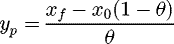 (6)
The flux equation for a component in a binary mixture is given by:
(6)
The flux equation for a component in a binary mixture is given by:
 (7)The first row of mesh cells in the feed side, and the permeate side considered sources. Introducing the negative source and source term at two sides of the membrane permits the gas to disappear from the feed domain via the membrane surface and emerge at the permeate side. The mesh was developed by using GAMBIT™. Grid size analysis is carried out using different mesh intervals. All the simulation results did not show any significant difference. The selected membrane mesh is shown in Figure 1. The mesh consists of 800 cells with the dimension of 0.05 m × 0.1 m.
FVM solver (ANSYS FLUENT™) solves the transport equation for a UDS in the same way as it solves the transport equation for a scalar in the core equations, such as a species mass fraction. The UDS capability can be used to implement a broad range of physical models. In this study, a model is developed to solve a general scalar diffusion equation (8) with the possible types of BCs at the boundary (or a part of the boundary) of the domain [24].
 (8)
(8)
The possible types of BCs are as follows:
 where Pc = PA/t, ∅ = plyp, φ∞ = phxf and D0, q0, φ∞ are constant values. The BC for left wall and the top wall is q = − Γ(∂ φ/∂ n = 0). The following equation gives mixed BC for right wall and the bottom wall.
 (9)
(9)
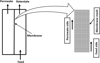 |
Fig. 1 Schematic representation and 2D mesh of a membrane. |
2.1 Steady-state modeling
Consider a steady-state scalar equation with constant Γ and zero sources term (Sφ = 0) as follows:
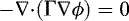 (10)
It is the Laplace’s equation. Solving the Laplace’s equation using the FVM UDS solver (ANSYS FLUENT™) does not necessarily require user-defined functions (UDFs). The graphical user interface is used to activate the UDS. FVM solver UDS provides only Dirichlet and Neumann conditions for the boundaries. Hence, the UDF applies on the mixed BC for the UDS equation.
(10)
It is the Laplace’s equation. Solving the Laplace’s equation using the FVM UDS solver (ANSYS FLUENT™) does not necessarily require user-defined functions (UDFs). The graphical user interface is used to activate the UDS. FVM solver UDS provides only Dirichlet and Neumann conditions for the boundaries. Hence, the UDF applies on the mixed BC for the UDS equation.
2.2 Formulation of mixed BCs
For a generic cell c0 adjacent to the boundary, the diffusive flux across the boundary face f of the cell expressed as follows:
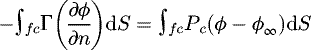 (11)
The diffusive flux by using the mid-point rule of surface integral approximation as:
(11)
The diffusive flux by using the mid-point rule of surface integral approximation as:
 (12)In FVM solver, the diffusive flux approximation is in two parts: in the first part, the first gradient is evaluated implicitly along the line connecting the cell centroid c0 to the centroid face f. It was corrected by a secondary gradient (or cross-diffusion) term evaluated explicitly by the gradient obtained from the previous iteration
  .
.
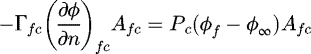
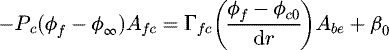
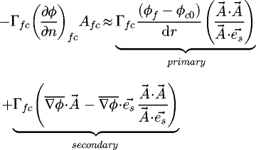 (13)FVM solver provides specific macros for UDF which define the necessary geometrical variables of the cell and calculate the secondary gradient term in equation (13). The secondary gradient term designated in equation (13), β0 and
  are defined as Abe. Hence, equations (12) and (13) can be written as:
 (14)φf can be expressed as follows:
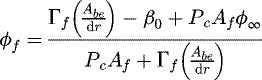 (15)The mixed BC for the UDS is ready to be specified by boundary profile φf in equation (15) through the UDF macro [25].
In most existing types of CFD software based on FVM, this kind of problem solved by introducing source terms which are known as user-defined functions (UDF). The correctness of CFD model is very sensitive to the source term which can disturb the flow position of neighboring cells in both feed and permeate domains (Fig. 2).
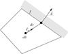 |
Fig. 2 Schematic of a cell adjacent to a boundary. |
3 Simulation setup and discretization
Table 1 shows values of different properties used in this research work. Figure 3 illustrates the solution procedure for a steady-state problem. A UDF was written in C programming language developed and compiled with FVM solver. The library functions based on UDF build and load during the execution of a CFD model. A mass transfer from hot air to a membrane is a problem that aligns with the grid, the numerical diffusion will indeed be small, and the first-order discretization scheme was implemented instead of the second-order scheme without any substantial loss of accuracy. The target of all discretization techniques like FVM is to develop a mathematical model to convert each of terms into an algebraic equation. Once implemented to complete control volumes in a mesh, a full linear system of equations was obtained that need to be solved. There are no standard criteria for examining convergence. Definitions of residual that are advantageous for one type of problem are occasionally deceptive for other types of problems. So, it is a good idea to examine convergence by judging residual stages besides observing related integrated quantities such as mass transfer coefficient. Intel Core™ i5 with 4 GB RAM is used to solve the steady-state problem. For steady-state problem, the CFD model was run for 100 iterations.
Values of different properties used in CFD modeling.
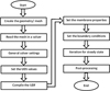 |
Fig. 3 Solution procedure for a steady-state problem. |
4 Results and discussion
The default convergence criterion for most problems in FVM solver (ANSYS FLUENT™) is satisfactory. The scaled residuals decrease to 10−3 as a standard of convergence for all equations except the mass, energy, for which the criterion is 10−6. Figure 4 illustrates the sum of facet values on permeate and retentate side at various points. ANSYS FLUENT™ is a cell-centered solver, so it stores data based on the cell-centered values. The only exception is BCs, which is stored in the facet centers. As the value of remains constant after 40 iterations (Fig. 4), the solution is considered as converged. Figure 5 shows that in this simulation the scaled residuals are decreased up to 10−8. Figure 6 demonstrates the flux through a polymeric membrane at various stage cuts in a steady-state problem [27]. The flux of the rectangular membrane from high to low values is clearly visible due to the use of mixed BC. It is observed that maximum diffusion occurs at the low value of stage cut. The proposed model results show a good agreement (±1–2%) with analytical values, particularly at low stage cuts (high feed rates). It illustrates the accuracy of the CFD model. Table 2 describes the values of binary gasses (oxygen and nitrogen) at permeate and retentate sides of a membrane. The maximum value of oxygen was achieved at the stage cut = 0.6 on the permeate side [28].
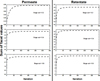 |
Fig. 4 Convergence history of sum of facet values on permeate and retentate side. |
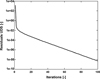 |
Fig. 5 Residuals profile of UDS. |
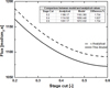 |
Fig. 6 Flux of oxygen through a polymeric membrane at various stage cuts. |
Fraction of binary gasses at permeate and retentate sides.
5 Conclusion
A CFD solution for mass transfer problem was formulated to examine the performance of the diffusion through the 2D rectangular membrane. The model was used to predict the steady-state problem in a membrane by solving the general scalar diffusion equation. The research focused on a diffusion process in a membrane due to a pressure gradient, which is useful in industries especially in chemical engineering. The FVM solver (ANSYS FLUENT™) provided the implementation of UDFs, which was written in the C programming language. These UDFs were compiled afterward for their use during solver execution for the solution of a problem. The residuals for the CFD model were decreased beyond the standard level to achieve more reliable results. The results for the problem showed that the developed CFD modeling approach could predict mass transfer in the polymeric membrane. More precise results can be obtained by applying the model to a 3D geometry with fewer assumptions.
This model can be extended to use for the modeling of complex gas mixtures as well as mass transfer problems to narrow the gap between laboratory and industrial scales.
Acknowledgments
The authors are grateful to Dr. Majid Ali, Centre for Advanced Studies in Energy (CAS − EN), National University of Sciences and Technology (NUST), Islamabad, Pakistan for his guidance and support during this research work.
References
- H.K. Versteeg, An introduction to computational fluid dynamics the finite volume method, 2/E, Pearson Education, India, 1995 [Google Scholar]
- J. Marriott, E. Sørensen, I. Bogle, Detailed mathematical modelling of membrane modules, Comput. Chem. Eng. 25 (2001) 693–700 [CrossRef] [Google Scholar]
- D.E. Wiley, D.F. Fletcher, Computational fluid dynamics modelling of flow and permeation for pressure-driven membrane processes, Desalination 145 (2002) 183–186 [CrossRef] [Google Scholar]
- E. Farno, M. Rezakazemi, T. Mohammadi, N. Kasiri, Ternary gas permeation through synthesized PDMS membranes: experimental and CFD simulation based on a sorption-dependent system using neural network model, Polym. Eng. Sci. 54 (2014) 215–226 [CrossRef] [Google Scholar]
- W.-H. Chen, C.-H. Lin, Y.-L. Lin, Flow-field design for improving hydrogen recovery in a palladium membrane tube, J. Membr. Sci. 472 (2014) 45–54 [CrossRef] [Google Scholar]
- R. Ghidossi, D. Veyret, P. Moulin, Computational fluid dynamics applied to membranes: state of the art and opportunities, Chem. Eng. Process.: Process Intensif. 45 (2006) 437–454 [CrossRef] [Google Scholar]
- L. Bao, G.G. Lipscomb, Well-developed mass transfer in axial flows through randomly packed fiber bundles with constant wall flux, Chem. Eng. Sci. 57 (2002) 125–132 [CrossRef] [Google Scholar]
- J.M. Gozálvez-Zafrilla, A. Santafé-Moros, S. Escolástico, J.M. Serra, Fluid dynamic modeling of oxygen permeation through mixed ionic-electronic conducting membranes, J. Membr. Sci. 378 (2011) 290–300 [CrossRef] [Google Scholar]
- M. Amokrane, D. Sadaoui, M. Dudeck, C.P. Koutsou, New spacer designs for the performance improvement of the zigzag spacer configuration in spiral-wound membrane modules, Desalin. Water Treat. 57 (2016) 5266–5274 [CrossRef] [Google Scholar]
- M. Ahsan, A. Hussain, Computational fluid dynamics (CFD) modeling of heat transfer in a polymeric membrane using finite volume method, J. Therm. Sci. 25 (2016) 564–570 [CrossRef] [Google Scholar]
- G.G. Lipscomb, S. Sonalkar, Sources of nonideal flow distribution and their effect on the performance of hollow fiber gas separation modules, Sep. Purif. Rev. 33 (2005) 41–76 [CrossRef] [Google Scholar]
- H. Takaba, S.-I. Nakao, Computational fluid dynamics study on concentration polarization in H2CO separation membranes, J. Membr. Sci. 249 (2005) 83–88 [CrossRef] [Google Scholar]
- M. Amokrane, D. Sadaoui, M. Dudeck, Effect of inter-filament distance on the improvement of reverse osmosis desalination process, S01 Modélisation avancée en mécanique des solides et des fluides, 2015 [Google Scholar]
- D. Fletcher, D. Wiley, A computational fluids dynamics study of buoyancy effects in reverse osmosis, J. Membr. Sci. 245 (2004) 175–181 [Google Scholar]
- Z. Cao, D. Wiley, A. Fane, CFD simulations of net-type turbulence promoters in a narrow channel, J. Membr. Sci. 185 (2001) 157–176 [CrossRef] [Google Scholar]
- V.T. Geraldes, V. Semião, M.N. de Pinho, Flow and mass transfer modelling of nanofiltration, J. Membr. Sci. 191 (2001) 109–128 [CrossRef] [Google Scholar]
- C. Koutsou, S. Yiantsios, A. Karabelas, Numerical simulation of the flow in a plane channel containing a periodic array of cylindrical turbulence promoters, J. Membr. Sci. 231 (2004) 81–90 [CrossRef] [Google Scholar]
- C. Koutsou, S. Yiantsios, A. Karabelas, Direct numerical simulation of flow in spacer-filled channels: effect of spacer geometrical characteristics, J. Membr. Sci. 291 (2007) 53–69 [CrossRef] [Google Scholar]
- T. Katoh, M. Tokumura, H. Yoshikawa, Y. Kawase, Dynamic simulation of multicomponent gas separation by hollow-fiber membrane module: nonideal mixing flows in permeate and residue sides using the tanks-in-series model, Sep. Purif. Technol. 76 (2011) 362–372 [CrossRef] [Google Scholar]
- W. Koros, G. Fleming, Membrane-based gas separation, J. Membr. Sci. 83 (1993) 1–80 [CrossRef] [Google Scholar]
- B. McLellan, E. Shoko, A. Dicks, J. Diniz da Costa, Hydrogen production and utilisation opportunities for Australia, Int. J. Hydrog. Energy 30 (2005) 669–679 [CrossRef] [Google Scholar]
- J. Zhang, D. Liu, M. He, H. Xu, W. Li, Experimental and simulation studies on concentration polarization in H2 enrichment by highly permeable and selective Pd membranes, J. Membr. Sci. 274 (2006) 83–91 [CrossRef] [Google Scholar]
- M. Abdel-Jawad, S. Gopalakrishnan, M. Duke, M. Macrossan, P.S. Schneider, J. Diniz da Costa, Flowfields on feed and permeate sides of tubular molecular sieving silica (MSS) membranes, J. Membr. Sci. 299 (2007) 229–235 [CrossRef] [Google Scholar]
- A. Fluent, Fluent 6.3 user guides: 8.6 User-Defined Scalar (UDS) diffusivity, Fluent Inc., USA, 2006, pp. 50–58 [Google Scholar]
- A. Fluent, Fluent 6.3 UDF manual, Fluent Inc., USA, 2006 [Google Scholar]
- R.W. Baker, Membrane technology and applications, third edition, Wiley, UK, 2004, pp. 325–378 [Google Scholar]
- M. Ahsan, A. Hussain, Mathematical modelling of membrane gas separation using the finite difference method, Pac. Sci. Rev. A: Nat. Sci. Eng. 18 (2016) 47–52 [Google Scholar]
- S.S. Hosseini, J.A. Dehkordi, P.K. Kundu, Gas permeation and separation in asymmetric hollow fiber membrane permeators: mathematical modeling, sensitivity analysis and optimization, Korean J. Chem. Eng. 33 (2016) 3085–3101 [CrossRef] [Google Scholar]
Cite this article as: M. Ahsan, A. Hussain, A computational fluid dynamics (CFD) approach for the modeling of flux in a polymeric membrane using finite volume method, Mechanics & Industry 18, 406 (2017)
All Tables
All Figures
|
Fig. 1 Schematic representation and 2D mesh of a membrane. |
| In the text | |
|
Fig. 2 Schematic of a cell adjacent to a boundary. |
| In the text | |
|
Fig. 3 Solution procedure for a steady-state problem. |
| In the text | |
|
Fig. 4 Convergence history of sum of facet values on permeate and retentate side. |
| In the text | |
|
Fig. 5 Residuals profile of UDS. |
| In the text | |
|
Fig. 6 Flux of oxygen through a polymeric membrane at various stage cuts. |
| In the text | |
Current usage metrics show cumulative count of Article Views (full-text article views including HTML views, PDF and ePub downloads, according to the available data) and Abstracts Views on Vision4Press platform.
Data correspond to usage on the plateform after 2015. The current usage metrics is available 48-96 hours after online publication and is updated daily on week days.
Initial download of the metrics may take a while.