| Issue |
Mechanics & Industry
Volume 22, 2021
Advances of junior researchers in aerospace sciences: a focus on innovative design
|
|
|---|---|---|
| Article Number | 39 | |
| Number of page(s) | 19 | |
| DOI | https://doi.org/10.1051/meca/2021037 | |
| Published online | 08 July 2021 | |
Regular Article
Tools and methodologies for box-wing aircraft conceptual aerodynamic design and aeromechanic analysis
1
University of Pisa - DICI, Via G.Caruso 8,
Pisa,
Italy
2
SkyBox Engineering, Via G.Caruso 8,
Pisa,
Italy
* e-mail: This email address is being protected from spambots. You need JavaScript enabled to view it.
Received:
30
July
2020
Accepted:
29
May
2021
Abstract
A way to face the challenge of moving towards a new greener aviation is to exploit disruptive aircraft architectures; one of the most promising concept is the PrandtlPlane, a box-wing aircraft based on the Prandtl's studies on multiplane lifting systems. A box-wing designed accordingly the Prandtl “best wing system” minimizes the induced drag for given lift and span, and thus it has the potential to reduce fuel consumption and noxious emissions. For disruptive aerodynamic concepts, physic-based aerodynamic design is needed from the very early stages of the design process, because of the lack of available statistical data; this paper describes two different in-house developed aerodynamic design tools for the PrandtlPlane conceptual aerodynamic design: AEROSTATE, for the design of the box-wing lifting system in cruise condition, and THeLMA, aiming to define the layout of control surfaces and high lift devices. These two tools have been extensively used to explore the feasible space for the aerodynamic design of the box-wing architecture, aiming to define preliminary correlations between performance and design variables, and guidelines to properly initialize the design process. As a result, relevant correlations have been identified between the rear-front wing loading ratio and the performance in cruise condition, and for the rear-front flap deflections and the aeromechanic characteristics in low speed condition.
Key words: Box-wing / disruptive configurations / innovation / future aviation / aircraft design / prandtlplane / parsifal
© K. Abu Salem et al., Published by EDP Sciences 2021
 This is an Open Access article distributed under the terms of the Creative Commons Attribution License (https://creativecommons.org/licenses/by/4.0), which permits unrestricted use, distribution, and reproduction in any medium, provided the original work is properly cited.
1 Introduction
The requirements for the aviation of the future are very ambitious and mainly concern the reduction of noxious emissions. The FlightPath2050 document [1] describes the European vision of the future air transportation and outlines the objectives to be achieved in commercial aviation sector; the main goal that has to be addressed is the drastic reduction of the aviation impact on climate change [2,3]; at the same time, the commercial aviation has to meet the expected huge increase in air traffic demand [4,5].
In addition to the incremental improvement of the state-of-the-art technologies currently used to design and produce transport aircraft, industry and research are exploring disruptive technologies, both in the field of propulsion and in the exploration of novel airframe configurations, to face these demanding challenges [6]. In the field of propulsion, major efforts are focused on the development of hybrid or electric propulsion systems [7–9], thus favouring the increasing use of electric energy or hydrogen in place of fossil fuels. As far as innovative configurations are concerned [10–12], different solutions have been proposed, and many of these are currently under study; the Blended Wing Body [13,14] and Joined Wing [15] configurations are worthy of mention in this field. These latter, such as diamond wings, strut/truss braced wings, and box-wing, have obtained considerable interest, as extensively described in [16]. The box-wing layout has been first indicated by Ludwig Prandtl in 1924 [17] as the “Best Wing System” which minimizes the induced drag for given lift and wingspan. Research performed since 1990s at University of Pisa has confirmed that a closed-form-solution of the minimum induced drag problem exists [18] and that it is possible to apply the Prandtl's concept to several aircraft categories [19], including both transport and leisure aircraft [20,21]. In Prandtl's honour, the aircraft architecture based on the “Best Wing System” has been called PrandtlPlane.
The PrandtlPlane has been object of study within the project PARSIFAL (“Prandtlplane ARchitecture for the Sustainable Improvement of Future AirpLanes”, [22,23]), which has been funded by the Horizon2020 programme and included University of Pisa (Italy), ONERA (France), TU Delft (Netherlands), DLR (Germany), SkyBox Engineering S.r.l. (Italy) and ENSAM (France) in the Consortium. Figure 1 shows an artistic representation of the PrandtlPlane configuration developed in PARSIFAL.
Since there are no statistical information, databases and empirical models regarding non-conventional configurations, it is necessary to develop specific procedures and tools for aircraft design and performance analysis; such physics-based tools need to be used from the early stages of the conceptual design of the aircraft, in order to provide design guidelines, to identify relevant correlations between design variables and performance, to select the proper design space for the further development of the aircraft. Therefore, the scope of this paper is to present some specific methods and tools for the aerodynamic analysis and design of the PrandtlPlane, to be used in the conceptual stage of the aerodynamic design. In the first part of this paper, a tool for conceptual sizing of the lifting system of box-wing configurations, called AEROSTATE, is presented; this tool has been conceived for the aerodynamic design of PrandtlPlane configurations considering the cruise conditions and has been adopted in several research projects such as IDINTOS (“IDrovolante Innovativo Toscano”, [20]) and PARSIFAL [22,24]. The AEROSTATE tool is based on a constrained aerodynamic optimization procedure and uses low-fidelity aerodynamic solvers to obtain a large amount of results and design information in a short time. Some general examples of AEROSTATE application are reported in order to describe how the tool works and which information for box-wing design can be obtained.
In the second part of the paper a tool for the conceptual sizing of control surfaces and high-lift systems, called THeLMA, is described. This tool performs two different tasks: in a first phase the sizing of control surfaces and flaps is carried out, considering the approach trim condition as reference; in the second part the selected configuration is analysed during the take-off, thanks to the simulation of the take-off dynamics coupled with the evaluation of the aerodynamic characteristics in ground effect.
 |
Fig. 1 PARSIFAL PrandtlPlane configuration. |
2 Aerodynamic design of the box-wing: the tool AEROSTATE
2.1 Overview
The high speed sizing for the PrandtlPlane lifting system is performed by means of the code AEROSTATE (“AERodynamic Optimization with STAtic stability and Trim Evaluator”); this code is written in MATLAB and has been developed at University of Pisa [25,26]. The AEROSTATE tool is based on a constrained aerodynamic optimization procedure, defined as follows: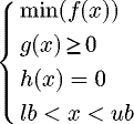 (1)
(1)
In the general optimization problem described in (1) x is design variables vector, whose components can vary into the design space defined by lower and upper boundaries, lb and ub respectively; f is the objective function to be minimized; g and h are sets of inequality and equality constraints.
The optimum configuration is searched in AEROSTATE by means of a combination of local analytical algorithms and global optimization methods; the two optimization strategies can qualitatively be described as follows:
Local algorithms: the search for the minimum is performed by means of analytical strategies, such as looking for the optimum solution in the direction of the maximum gradient. These algorithms are named local methods because the procedure finishes as the first minimum is found, and it is strictly dependent from the initial starting point; in principle it is not ensured that the solution found by these methods is the overall minimum. However, the solution found is better than the starting point. These methods are efficient, as they require reduced computation effort, but they are not effective, as they do not guarantee the search for the global optimum.
Global algorithms: these algorithms typically parameterize the design space in subdomains in order to identify the design space area where the global minimum solution is present. By means of these algorithms, it is possible to have the confidence to have explored the whole feasible domain, and to have identified the global optimum. The effectiveness of such methods, however, is accompanied by a considerable increase in computation effort compared to analytical algorithms.
There is also a third strategy to deal with optimization problems, that provides for using a combination of local and global optimization algorithms to get the advantages from both methods: efficiency of local search strategy and effectiveness of global optimization. In AEROSTATE a mixed strategy that combines global and local optimization algorithms has been implemented; in particular, the Sequential Quadratic Programming “SQP” [27,28] has been used as local algorithm, whereas the “LocalSmooth” [26,29] algorithm has been implemented as global optimizer. The strategy adopted in “LocalSmooth” of using the “SQP” local algorithm to find the global optimum is described in the following of this section. The AEROSTATE aerodynamic optimization is written in MATLAB; the software structure is modular so that other algorithms for the local optimization can be used or other aspects regarding the aircraft design can be implemented.
The aerodynamic solver used in AEROSTATE is the Vortex Lattice Method code AVL [30], that in a very short time allows to examine a large number of configurations, and so to identify relevant trends between performance and design variables; this is very useful in the conceptual design stage and allows to identify starting promising solutions for the following detailed development with higher fidelity tools and methodologies. Due to the limitations of the potential aerodynamic solver, especially for the transonic conditions, a calibration of the boundaries of the design space and a proper tuning of the aerodynamic constraints (i.e. maximum values of local spanwise lift coefficient) may be useful for specific design studies, as has been done in [24], by using the information collected in transonic CFD campaigns [31,32].
The AEROSTATE code is mainly divided in three macro-blocks: the pre-processing set up, the optimization process, and the post-processing of the results (Fig. 2).
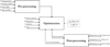 |
Fig. 2 General scheme of AEROSTATE architecture. |
2.2 Pre-processing phase
In the first phase, the pre-processing, the designer sets the optimization problem by defining the initial starting point, the optimization variables, the design space, the constraints, and all the information necessary to initialize and perform the aerodynamic evaluations. In particular:
The initial starting point x0 is represented by a random geometry of the aircraft lifting system planform; all the geometric information to define the configuration are collected in MATLAB structure, that allows to easily define the geometry of multiplanes by using different structure sub-levels.
The optimization variables are generally related to the lifting system planform geometry; in particular, for a generic multiplane of n-wings, the design variables for each wing identified by i-sections and j-bays (j = i ‑ 1) are: ci (chord), θi (twist angle), xLEi (longitudinal leading edge position), Λj (sweep angle), Γj (dihedral), bj (span). The design space is then defined by properly setting the boundaries to each design variables (i.e. lower boundary lb and upper boundary ub, in Eq. (1)), accordingly to each specific design case. The sections airfoils are not considered as design variables.
The optimization constraints can be related to several aspects of the aerodynamic design; specifically, it is possible to set constraints regarding the aerodynamics, the flight mechanics, the geometry. In general, a complete set of constraint for the conceptual aircraft aerodynamic optimization can be summarized as follows:
-
Vertical trim, expressed as:
 (2)
(2)where L is the total lift generated by the aircraft, Wdes is the reference weight to be trimmed in the selected operating condition, and ϵL is a tolerance properly set accordingly to the degree of confidence regarding the design weight estimation.
-
Longitudinal static stability, expressed as:
 (3)
(3)where SSM is the Static Stability Margin, that is constrained between a maximum and a minimum value; the Static Stability Margin is defined as follows:
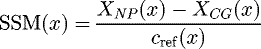 (4)
(4)where XNP and XCG are the longitudinal positions of the Neutral Point and of the Centre of Gravity, respectively, and cref is a reference chord.
-
Pitch trim, expressed as:
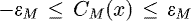 (5)
(5)where CM is the pitching moment coefficient, that is constrained to be equal to zero in the reference operating condition, apart from a tolerance ϵM, representative of the possibility to trim the aircraft by means of elevator deflections (not considered in these analyses).
-
Constraint on maximum local lift coefficient:
 (6)
(6)this relation constrains the lift coefficient of each section
 spanwise to be lower than a threshold value
  . When dealing with the aerodynamic design of a low subsonic aircraft, this threshold value is related to the airfoil maximum lift coefficient (
 , where SF is a safety factor); if a transonic aircraft is concerned, the
  has to be properly calibrated by considering the transonic performance of the airfoil [24], to avoid wave drag rise that is undetectable by using potential solvers.
 -
Limitations on wings loading:
 (7)
(7)where (L(x)wing/S(x)wing) is the wing loading of the nth wing of a multiplane, so the equation (7) represents a system of n equations, that constraints the wing loading for each lifting surface. The wing loading is a fundamental parameter in conceptual aircraft design, that influences directly aerodynamic performance as well as aeromechanical features, as described in Sections 2.5.1 and 2.5.2. For a box-wing configuration, the convention used to identify the wings reference surfaces S(x)wing is represented in Figure 3; the aircraft reference surface is defined then as Sref = Sfront + Srear.
-
Geometrical constraints, e.g.:
 (8)
(8)
 (9)
(9)where equation (8) fixes the taper ratio of each jth wing-bay to be lower than one; the equation (9) represents a geometric constraint specific for a box-wing: the position of the front wingtip is constrained to be spaced of a value Δx with respect to the rear wingtip, to satisfy specific design requirements (e.g. a proper vertical wing-tip sweep angle to avoid transonic phenomena, or to avoid complex structural solutions).
-
The set of constraints can be enriched with more relationships, or restricted to more simplified problems, according to the specific design case to be addressed.
The optimization procedure needs other inputs to initialize and perform the aerodynamic and aeromechanic computations; in particular:
-
Aircraft design weight, expressed as:
 (10)
(10)the operative empty weight Weo is evaluated by means of simplified literature methods, as proposed in [33], the fuel weight is evaluated through Breguet equations, and the payload weight through a statistical estimation [34].
Reference mission and operating conditions, in terms of range, altitude and cruise Mach number; as it has been chosen to model the fuselage in AVL as a lifting surface, the reference angle of attack is fixed for each computation equal to zero.
-
Airfoil drag polar curves, expressed as:
 (11)
(11)that is necessary to evaluate the parasite drag of the lifting system CD0; as the VLM solver is not able to evaluate viscous forces, a simple method based on the airfoil drag polars is implemented in AEROSTATE; the CD0 wing is evaluated for each lifting surface by integrating the CD foil (known on each ith section according to Eq. (11)) spanwise along the jth bay, according to the relation:
 (12)
(12) -
The total parasite drag of the a wing is:
 (13)
(13)and, in the case of the box-wing, the total lifting system parasite drag can be easily obtained from the equation (14):
 (14)
(14) -
Simplified fuselage geometry information, such as fuselage length Lfus, and fuselage equivalent diameter Dfus, to estimate the fuselage wetted surface Sfus and consequently the fuselage parasite drag CD0 fus through the formula proposed in [33]:
 (15)
(15)where the interference factor Q, the friction coefficient cf, and the form factor FF can be calculated using the relationships in [33].
In this way, the overall drag coefficient of the aircraft is calculated by the formula:
 (16)
(16)as the induced drag coefficient CDi is computed by AVL. If it is needed it is possible to take wave drag coefficient into account through the simplified Korn-Locke formula [35].
-
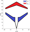 |
Fig. 3 Conventional definition of box-wing reference surfaces. |
2.3 Optimization strategy
As the pre-processor inputs are set, the optimization can be launched; the objective function f to be minimized is the opposite value of the lift-to-drag ratio (or aerodynamic efficiency), evaluated in cruise condition. For each optimization iteration the AVL code is called to compute the aerodynamic characteristics of the current configuration, to assess:
Induced drag coefficient CDi, to evaluate the objective function;
Lift coefficient CL and pitching moment coefficient CM, to assess the trim constrains;
The spanwise lift coefficient distribution, to check the constraint on local threshold cl(y);
Stability derivatives CLα and CMα, and so the longitudinal position of the neutral point XNP to assess the longitudinal stability constraint.
As the pitch trim and the static longitudinal stability depend both from aeromechanic characteristics and aircraft balance, during the optimization process the longitudinal position of the centre of gravity XCG is updated at each iteration; to take the weights of all the aircraft components into account, such as engines, lifting surfaces, fuselage, landing gear, etc., the weight estimation method presented in [36] has been implemented.
The global optimization procedure (Fig. 4) is initialized by sampling the design space into K starting points around the initial input geometry x0, and finding for each the local minimum, by means of the SQP method (initialization phase); then, the global algorithm interpolates the K local optima and finds a smoothed function of the local minima; the minimum of this function (current* configuration, representing the xlocal* solution) is considered as provisional global optimum (current* = record configuration) and is taken as a new starting point of the local optimization. The sampling of the design space is iterated around this point, and a new local optimization i is performed. If the optimizer finds a new local optimum (current configuration, described by the ith xlocal solution) that exhibits a minimum lower than the previous provisional global optimum, it sets currenti = record (thus, defining the new provisional global optimum), and again the procedure is iterated; else, if the local optimum is higher than the record, the optimizer moves to another sampled starting point (i = i+1) and again a new local optimization is performed. The procedure is iterated until all the sampled starting points are analysed (i = K); then, if any of the ith local minima is lower than record, the optimizer identifies the new current* configuration with the minimum of ith local minima and iterates the procedure (displacement phase). When a new current* configuration is set, with f(current*) > f(record), the algorithms counts the no improvement parameter NoImpr=NoImpr +1; the procedure is stopped when no improvements are observed within the maximum number of search attempts Nmax set in the pre-processor, and the last record configuration coincides with the global optimum. The detailed description of the mathematics of the procedure is described in [26,37,38].
A constraint violation threshold can be set in the optimizer; this is mainly needed in the exploration phase (Fig. 2) to avoid the solver does not find any solution, as −in the very first attempts of a specific design case- the designer does not know specifically the feasible boundaries of the design space. This constraint violation tolerance is also useful to strengthen or weaken individual constraints. With this strategy, if the optimization algorithm does not find feasible solutions (i.e. there is no feasible region in the design space), a solution is found in the unfeasible region (by violating one or more constraints) within a prescribed constraint violation tolerance; as an output, the optimizer provides the optimal solution, the value of the objective function, and the related degree of unfeasibility (i.e. the maximum constraint violation), if any.
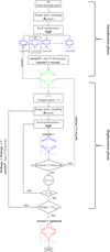 |
Fig. 4 Schematic representation of the global optimization algorithm. |
2.4 Post-processing phase
As a result of the combined use of local and global procedures, the output of each AEROSTATE run is composed of a group of configurations, as reported in a generic example in Figure 5, that shows the top and the front views of each aerodynamic design; namely, the blue configurations represent the local minima (current configuration), the green configurations represent provisional global minima (record configuration) and the red configuration is the global optimum of the whole procedure. Figure 6 shows a single configuration more in detail.
As AEROSTATE allows to obtain several groups of different aerodynamic designs, it can be used for different specific aims; in particular:
To explore wide design spaces, in order to identify the basic features of a specific architecture and to find trends between the performance and the main macro design variables; in these analyses the boundaries of the design space are preferably wide, and the constraints and the related tolerances are not to strict, to allow the most comprehensive exploration possible;
To initialize a design case, with the aim to define a set of configurations to be analysed more in detail in the following design stages;
To refine a starting configuration considering a restricted design space, to maximise its aerodynamic performance; as the information of the starting point are supposed to be detailed, the constraints and the tolerance can be more rigorous.
In this paper the first application will be presented; in particular, qualitative examples of using the AEROSTATE tool to obtain general information about the design of a transport box-wing aircraft is described; specifically, the effects of the global wing loading and the ratio between the front and rear wing loadings are taken into account as main parameters.
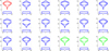 |
Fig. 5 Example of output of AEROSTATE. |
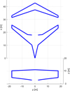 |
Fig. 6 Single AEROSTATE output configuration. |
2.5 Box-wing planform design and analysis through AEROSTATE
2.5.1 Influence of the global wing loading on the box-wing design
The influence of the global wing loading Wdes/Sref on the box-wing design has been assessed through an explorative design campaign by means of AEROSTATE, focusing on the effects of the global wing loading on the box-wing lift-to-drag ratio, or aerodynamic efficiency, hereafter indicated as E.
Such analyses have been performed considering the set of reference Top Level Aircraft Requirements (TLARs) indicated in Table 1, typical of a short-to-medium haul transport aircraft with the exception of the number of passengers (that is below 240 for conventional aircraft).
The design variables are those related to the lifting system geometry, such as chords c, twist angles θ, leading edge longitudinal position X, for the relevant wing sections, and sweep angles Λ, span b, dihedral angles Γ, for the corresponding wing bays; the design variables selected for this study are represented in Figure 7, and the related boundaries defining the design space are reported in Table 2.
In this example, the AEROSTATE tool has been used to generate families of configurations compliant with the constraints described by equations (2)‑(9); the values of the constraints imposed to this explorative design campaign are summarized in Table 3.
As Table 3 shows, three different maximum values of wing loading have been used to generate three different families of solutions. Figure 8 presents the results for the three runs of AEROSTATE in terms of percentage variations of lift-to-drag ratio (namely the aerodynamic efficiency E) versus the global wing loading; the percentage variations are evaluated with respect to the lowest value found during the process, in order to highlight the effect of the considered design variable in this parametric explorative analysis. Each marker type is assigned to a family of solutions, and each marker represents a designed configuration.
Since each solution is obtained for the same design weight according to equation (2), Figure 8 indicates that the improvement of aerodynamic efficiency in configurations with higher wing loading values is associated to the reduction of the total wing area. This is detailed in Figure 9, where the left chart quantifies the reduction of the reference surface, and so of the wetted surface, in solutions with higher global wing loading, whereas the right chart shows the associated reduction of total drag, mainly related to the parasite drag reduction.
The optimization of the aerodynamic efficiency is subject to the trim and stability constraints; in Figures 10 and 11 the results in terms of longitudinal stability margin and pitching moment are displayed, highlighting the fact that the constraints are satisfied within the prescribed tolerances reported in Table 3 for the configurations evaluated.
In order to satisfy these constraints, the optimization algorithm acts on the repartition of the wing loading between front and rear wing; the wing loading of each surface is defined as the lift generated by each wing divided by the corresponding wing surface, as described by the following equations: (17)
(17)
 (18)
(18)
In this case, in which the ratio between the front and rear wing loading is unconstrained, the optimization algorithm finds that all solutions tend to reach the maximum wing loading admissible for the front wing, having a lower value for the rear wing. As Figure 12 shows, the ratio between the rear and the front wing loading is in the range 0.6‑0.67 for the solutions described in this paragraph.
The information from this example provide a general picture of the trends that can be identified through the proposed approach, which can be very useful in the early stages of the design process; the designer can use the AEROSTATE tool iteratively modifying the inputs, the constraints and the design space in order to achieve the solutions that more satisfy the design requirements; an example of PrandtlPlane design initialized with the AEROSTATE tool is given in [39,40].
Reference TLARs.
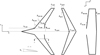 |
Fig. 7 Design variables selected for the case study. |
Design space for the case study.
Optimization constraints values.
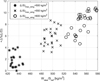 |
Fig. 8 Lift-to-drag trend vs global wing loading. |
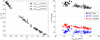 |
Fig. 9 Reference surface vs lift coefficient (left); total drag vs varying global wing loading (right). |
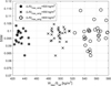 |
Fig. 10 Longitudinal static stability margin vs global wing loading. |
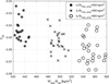 |
Fig. 11 Pitching moment coefficient vs global wing loading. |
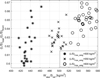 |
Fig. 12 Rear −front wing loading ratio vs global wing loading. |
2.5.2 Influence of the front-rear wing loading repartition on the box-wing design
In order to generally describe the role of the rear wing aerodynamic design into the whole design process of a box-wing aircraft, another constraint has been added to the constraint set of the previous example. As said in the previous section, the lift-to-drag ratio improves when the global wing loading increases; due to the fact that the front wing loading, in the cases of interest, reaches the maximum value allowable (and not being able to increase significantly this value because of the drag rise problems [24,31]) that cannot be detected by a potential aerodynamic solver, as AVL), the only way to increase the global wing loading is to increase the rear wing loading. Thus, a new constraint is included (Eq. (19)): (19)where Rmin is the minimum prescribed value for the wing loading ratio. In the next example, the following three values are assigned to Rmin: 0.5, 0.8 and 1.0. In addition, any wing cannot exceed the maximum wing loading arbitrarily set equal to 550 kg/m2. As expected, by increasing the ratio of the wing loadings, an increase of the global wing loading follows as well, together with an improvement of the aerodynamic efficiency, as reported in Figure 13.
However, the increase of the rear-front wing loading ratio has negative effects on longitudinal stability and equilibrium. In fact, Figure 14 shows that the static stability margin moves from positive to negative values, as the wing loading ratio is increased beyond the upper limit of the typical range shown in Figure 12. In addition, Figure 15 underlines how larger wing loading ratios are associated to larger pitching moments, hence more demanding in terms of elevators size and/or deflections.
These results indicate that the aerodynamic design of the lifting system needs a trade-off among the requirements of flight mechanics (i.e. stability, trim) and aerodynamic performance (i.e. lift-to-drag ratio). In particular, the ratio between the rear and front wing loading is a fundamental parameter for the design of a box-wing configuration; specifically, it has a key role to manage the contrast between static stability and pitch trim: e.g., as for the box-wing the reference position of centre of gravity is closer to the front wing, the critical condition for the pitch equilibrium is the lift repartition between rear and front wing Lrear/Lfront, and a larger lift is needed on the front wing (Fig. 16); the stability requirements imposes to the rear surface to be adequate to guarantee the proper margin of stability. Both the conditions force to design a rear wing less loaded than the front wing.
As said before, by changing the constraints and the design space boundaries in the AEROSTATE tool, the designer can force the procedure to obtain specific solutions or to collect information on configurations far from the set of the optimal ones. In the previous example, the configurations with minimum rear-front wing loading ratios constraint equal to 0.8 and 1 showed, in general, a negative SSM, that is an unacceptable condition for designing civil aircraft.
In order to better understand the effects of the rear-front wing loading ratio on longitudinal stability and trim, AEROSTATE has been used to design longitudinally stable configurations while the pitch trim constraint has been relaxed. In detail, three families of solutions have been generated fixing the rear-front wing loading ratio constraint equal to 1, each of them fulfilling the constraints listed in Table 3 with the only exception of the pitching moment one which has been gradually relaxed; Figure 17 shows that when this constraint is relaxed, the optimization algorithm can find stable solutions.
As a general guideline, increasing the unbalanced pitching moment to improve the SSM in not a good strategy, since large elevator deflections may be needed for a long stage of the cruise to restore the pitch equilibrium condition, with negative effects on the aerodynamic efficiency due to the increase of the trim drag.
The information achievable through AEROSTATE, even though the tool is based on a low-fidelity aerodynamic solver, are useful to initialize the design process; as shown in the general examples described in this paragraph, the tool can provide some relevant design guidelines and relevant trends between performances and design variables. In particular, for a box-wing architecture, the front wing needs a higher wing loading with respect to the rear wing, to satisfy stability and trim requirements. In a very early design phase, the ratio between the rear wing loading and the front wing loading may assume values in the range 0.5‑0.8, to define a proper design space. The wing loading repartition implies that the whole configuration exhibits performance penalties in terms of aerodynamic efficiency with respect to the unconstrained configurations; this, because of the overall wing loading reduction due to a more unloaded rear wing.
Of course, the preliminary results obtained by the AEROSTATE tool must be implemented with other results coming from the different disciplines concurring to the aircraft design process, and with more refined tools. For example, the correlation of the rear-front wing loading ratio with the aerodynamic efficiency and stability must be coupled with more reliable structural sizing and weight prediction models. In this way, it is possible to provide a more accurate positioning of the lifting surfaces and of the centre of gravity.
Constraints coming from low speed flight must be considered as well; for example, having high values of rear-front wing loading ratio is unfavourable for the stall condition; in fact, having a more loaded front wing, and so being in principle this lifting surface more critical with respect to the stall, can confer to the box-wing its typical ‘anti-stall’ behaviour, as shown by numerical and wind-tunnel test campaign [21], and qualitatively represented in Figure 18.
As the stall condition is reached, the flow separation starts on front wing, while the rear wing is still generating lift; this introduces an increase of the negative pitching moment contrasting the stall condition.
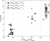 |
Fig. 13 Aerodynamic efficiency vs rear-front wing loading repartition. |
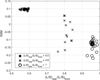 |
Fig. 14 Longitudinal static stability margin vs rear-front wing loading repartition. |
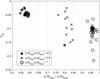 |
Fig. 15 Pitching moment vs rear-front wing loading repartition. |
 |
Fig. 16 Pitch trim scheme for a box-wing. |
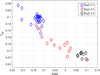 |
Fig. 17 Longitudinal static stability margin vs pitching moment. |
 |
Fig. 18 PrandtlPlane ‘anti-stall’ behaviour. |
3 Design of control surfaces: the THeLMA tool
The low speed analysis for the box-wing configuration has been performed by the in-house tool THeLMA (“Tool for High-lift and Movable surfaces Analysis”); the code, written in MATLAB, uses a simplified procedure to size the movable surfaces and high-lift systems of the box-wing, and to analyse the aeromechanical behaviour and performance of the aircraft in approach and take-off phases. According to the literature on the PrandtlPlane [21,41,42], the reference layout assumed for the control surfaces is characterized by counter-rotating elevators placed at the root zones of both wings, ailerons placed at the tip regions and trailing edge flaps placed in the intermediate zones (Fig. 19).
In a first step, the THeLMA code performs the preliminary sizing of control surfaces and high-lift devices for a generic input configuration, considering the approach flight condition; in a second step, the simulation of the take-off manoeuvre is performed. As for the sizing of the lifting surfaces described in Section 2, in this case the purpose of the procedure is to obtain design indications in the very early stage and to obtain correlations between performance and main design parameters for the box-wing in low speed condition. In order to get quick results on a high number of configurations, THeLMA uses AVL as aerodynamic solver.
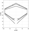 |
Fig. 19 Reference PrandtlPlane configuration: sketch of movables layout. |
3.1 Approach condition: preliminary sizing of high-lift devices and control surfaces
A preliminary sizing procedure for both elevators and flaps has been defined in approach condition, considering the reference layout for the box-wing movables. In order to detect the available span for flaps and elevators, the procedure is initialized with a first sizing of the ailerons. In this conceptual stage, the aileron effectiveness is evaluated in terms of capability to set the aircraft to a required roll angle  . An approximated one degree of freedom roll dynamic is used to evaluate the steady value of roll angle ϕ∞, considering the aileron input as an impulsive function. Given an initial guess for the ailerons' span, the AVL code is used to evaluate the aileron control derivative Clδa, and consequently to calculate the steady roll angle ϕ∞. If
  the aileron span is iteratively increased, until the requirement is satisfied.
Once the span required for the ailerons has been defined, the remaining wings span can be used to initialize elevators and trailing edge high-lift systems, and the general approach trim problem (defined in Eq. (20)) can be solved: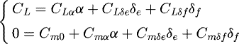 (20)
(20)
The trim problem is solved by using AVL code; in particular the angle of attack (αtrim) and the elevators deflection (δe trim) are calculated by the solver in order to satisfy the pitch moment trim (CM = 0) and the vertical trim (CL = CL approach), as the front and rear flap deflections are provided as input. The aeromechanical characteristics of the flapped configurations, as maximum lift coefficient CL MAX and stall speed, are fundamental to define the approach conditions; a simplified iterative procedure for the CL max assessment of the flapped box-wing aircraft has been defined as follows:
The stall characteristics of each flapped lifting surface, depending to the selected high-lift system, are evaluated with the methods described in [43];
For each front and rear flap deflections, the stall-critical wing is identified by evaluating the value ΔCL crit wing = CL MAX wing ‑ CL wing, where CL MAX wing is the maximum lift coefficient of each wing evaluated by means of the method in [43], and CL wing is the current lift coefficient of each wing evaluated by AVL for the low speed trim condition; the critical wing is the one with the lowest value of ΔCLcrit wing;
Then, using AVL, the angle of attack of the aircraft is iteratively varied until the condition CL wing = CL MAX wing is reached; in correspondence of this condition, the CL of the aircraft coincides with the global CL MAX, with which it is possible to calculate the stall speed, and therefore the approach speed.
The simplified procedure for elevators and flaps sizing is schematically represented in Figure 20, and can be summarized in the following points:
First, the ailerons are sized, and the span available for the elevators and flaps is identified;
Flaps and elevators are initialized;
Approach performance (CL MAX, Vstall) of the flapped configuration are estimated;
Trim problem's is solved;
If the trim δe exceed a threshold fixed by the designer, the elevators' span is increased, and consequently the flap span is reduced, causing a variation in the approach performance of the flapped box-wing;
Iteratively, the performances are updated and the new trim condition is evaluated, until the constraint on the elevators' deflection is satisfied;
A stall check of the output configuration is performed by comparing the lift coefficient spanwise distribution with the Cl max of the flapped airfoil.
For each box-wing analysed by THeLMA code, several combinations of front-rear flap deflections are considered, in order to identify the influence of the two flapped wings on both low speed performance and trim requirements; the parameter Flap Gain (FG) has been defined as in equation (21), to evaluate the different effects of the rear and front flap deflections: (21)
(21)
In the following, the front flap deflection is indicated with the symbol δflap, as the parameter FG is used to refer to the related rear flap deflection.
Some general considerations regarding the conceptual design of the high-lift systems and the analysis of the low speed performance of PrandtlPlane are discussed in the following. A parametric exploration by means of THeLMA tool provides information on the low speed characteristics of PrandtlPlane and on its aeromechanical features. In particular, a sensitivity analysis with respect to the main design parameters δflap and FG is discussed, taking a reference PrandtlPlane configuration (Fig. 19) into account. The lifting system of this configuration has been designed by means of AEROSTATE tool, according to the requirements reported in Table 1 and the constraints in Table 3; the configuration exhibits a rear-front wing loading ratio equal to 0.61: the rear-front wing loading ratio is a fundamental parameter that also affects the low speed performance of the clean and flapped lifting system. For both wings single slotted fowler flaps have been considered as trailing edge high-lift devices. It is worth underlining that the discussion on the results about the low speed characteristics of this configuration is intended to provide qualitative guidelines and indications on the aeromechanical behaviour of the box-wing lifting system architecture.
The preliminary results for the reference configuration are presented in terms of low speed performance (Figs. 21 and 22) and trim parameters (Figs. 23 and 24). Figure 21 shows that the most relevant approach performance criterion, the CL MAX, depends largely on the deflection of the front flap and is almost independent of the deflection of the rear flap. Increasing the FG, in fact, the CL MAX rear increases keeping the rear wing far from the stall condition; however, the rear wing is not critical for a box-wing designed according the indications presented in Section 2, and so this improvement does not affect the aircraft global CL MAX (Fig. 21). Indeed, Figure 22 (left) shows the ΔCL crit-front values which are lower than ΔCL crit rear (Fig. 22 (right)) for all the combinations of δflap and FG. The CL MAX directly affects the stall speed Vstall, and therefore the approach speed (Vapp = 1.3 Vstall).
It can be observed that the rear wing is never critical in terms of stall occurrence for any combination of flaps settings (front and rear), and moreover there is a significant ΔCL crit wing gap between the front and rear wing; it suggests that the technology of the rear high-lift devices may be simplified with respect the front one.
On the other hand, one of the main effects of deflecting the rear flap concerns the approach trim; analysing the graphs related to the trim parameters in Figures 23 and 24, it can be observed that: (a) the rear flap deflection has limited impact on CL trim (Fig. 23); (b) by fixing δe = 0° (and so, the aerodynamic solver does not search the pitch trim by means of the elevators deflection), it can be observed that the rear flap deflection can be used to provide pitch equilibrium (CM trim = 0, Fig. 24 (left)), generally without loss of performance at low speed in terms of CL MAX (Fig. 21 (left)): this theoretically allows the elevators to be not deflected in the ideal case of CM = f(δflap, FG) = 0, as shown in Figure 24 (right).
To summarize, general conceptual design guidelines related to the sizing of high-lift systems for box-wing can be addressed by the previous discussion; namely:
If the box-wing is sized consistently with the requirements of aerodynamic efficiency, longitudinal static stability, pitch trim and stable stall, the critical wing with respect to the stall in low speed condition is the front one.
The overall low speed performance of the aircraft (i.e. CL MAX) is directly related to the performance of the flapped front wing, while the rear wing high-lift devices have a marginal influence.
The rear wing flaps are necessary to properly provide the aircraft pitch trim.
However, since the performance of the flapped rear wing has no influence on the global performance, it is possible to size the rear wing high-lift devices considering technologies much simpler than the front wing; the rear wing high-lift devices must also guarantee that the rear wing is never critical to the stall, in order to avoid unacceptable problems of unstable stalling.
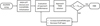 |
Fig. 20 Sketch of movables/high-lift devices sizing process. |
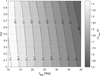 |
Fig. 21 CL MAX varying δflap front and FG. |
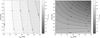 |
Fig. 22 ΔCL crit front (left) and ΔCLcrit rear (right) varying δflap front and FG. |
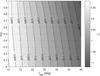 |
Fig. 23 Trim lift coefficient in approach varying δflap front and FG. |
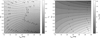 |
Fig. 24 Pitching moment @ δe = 0°, left; Elevator deflection δe to reach the approach pitch trim, right. |
3.2 Take-off manoeuvre simulation and analysis
The approach described in [44] for the simulation of the take-off dynamics has been implemented in THeLMA, and here adopted for the specific case of box-wing architectures, in order to expand the knowledge on control surfaces and high lift devices design.
The take-off manoeuvre is divided in three phases (ground roll, rotation and lift off), and the simulation of the dynamics is performed by integrating the differential equations of motion using the Euler method. The aerodynamic characteristics are evaluated in each time-step by means of AVL, taking the ground effect into account. This latter aspect is of great importance in the case of the box-wing since both the ‘air cushion’ effect, which increases the lift, and the ‘vortex breakdown’, which reduces the induced drag, depend on the distance of the lifting surfaces to the ground and to the aircraft attitude. The AVL code allows to evaluate these effects in a simplified but fast way; the trailing-edge high-lift devices are modelled as plain flap. The parasite drag of the fuselage is evaluated by means of the method described in Section 2, as well as the drag of the landing gear and high-lift devices is estimated as proposed in [45]. More details on the PrandtlPlane performance in ground effect and on the take-off dynamic simulation are reported in [44].
In this paragraph some qualitative trends of the performance of a box-wing aircraft related to front flap deflection δflap and the Flap Gain (FG) are discussed, taking the reference configuration in Figure 19 into account.
The take-off simulations have been performed under the following assumptions: full thrust for the two engines for the entire manoeuvre; dry runway; no wind during the take-off; airport at sea level; standard air condition.
Results are reported in Figure 25, showing the take-off runway length XTO (left) and speed at the end of the manoeuvre Vobstacle (right), as function of δflap and FG; as expected, the runway length requested for the take-off decreases when the δflap increases. This is intuitive because, as the front flap deflection increases, the global CL MAX Figure 21 increases and consequently the take-off stall speed decreases.
A less explicit relationship exists between take-off performance and Flap Gain; the results show that higher FG values, i.e. larger deflections of the rear flap, increase the runway length required. In fact, a positive rear flap deflection, while having negligible effects on aircraft CL MAX (Fig. 21), introduces a negative contribution to the pitch moment, in opposition to the elevator action necessary to rotate the aircraft; consequently, large values of Flap Gain penalize the take-off run length. The opposite occurs as δflap increases and Flap Gain decreases: the initial ground-roll pitching moment coefficient CM rull of the aircraft turns positive (Fig. 26 (left)), and therefore the aircraft experiences a natural pull-up moment during the take-off run (Fig. 26 (right)). This aspect is peculiar of the PrandtlPlane configuration, due to the two lifting surfaces sufficiently far from the centre of gravity.
Reducing FG can make the aircraft naturally pull-up (CM rull > 0), causing the anticipation of aircraft rotation even before the activation of the elevators (Fig. 26), and consequently the reduction of runway length. Nevertheless, this could lead to a considerable anticipation of the actual rotation speed, even lower than the V1 decision speed, compromising the compliance of the manoeuvre with regulatory requirements; this must be taken into account in the development phases of a box-wing configuration, properly calibrating the couple δflap-FG with respect to the specific aircraft weight and balance.
The results here reposted show how the THeLMA tool can produce some preliminary design indications also for the take-off phase; varying the input configuration and the design parameters, the designer can collect information and guidelines on several aeromechanical and aerodynamic features of the box-wing. Of course, during the aircraft design process, these guidelines must be integrated with results and outputs coming from higher fidelity tools, such as CFD assessment for the aerodynamic performance.
 |
Fig. 25 Take-off runaway length (left) and final speed (right). |
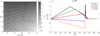 |
Fig. 26 Ground roll aerodynamic pitching moment coefficient (left); aerodynamic moment evolution during take-off (right). |
4 Conclusions
In this paper methods to obtain conceptual aerodynamic design guidelines for the unconventional box-wing lifting system have been presented; these procedures rely on design tools specifically developed for this unconventional airframe, that are described in the paper: AEROSTATE, which aims to size the lifting system of box-wing configurations and is based on an aerodynamic optimization procedure, and THeLMA, which allows to define the layout of control surfaces and high-lift devices considering the approach trim condition, as well as to analyse the performances during the take-off manoeuvre. Both the tools adopts a VLM solver to reduce computational costs. These tools are useful to obtain design guidelines and trends between the box-wing design parameters and main aerodynamic and aeromechanical performances. As relevant examples, AEROSTATE has been used to identify the trade-off between the cruise aerodynamic performance and the stability and trim requirements typical of the box-wing architecture; the global wing loading and its repartition among front and rear wings play a key role in managing this trade-off, by affecting aerodynamic and flight mechanics characteristics such as lift-to-drag ratio, longitudinal static stability margin and pitching moment. In particular, it is worth to remark how the achieved results indicate that to design a box-wing that satisfies the longitudinal trim and stability requirements it is necessary to properly reduce the rear wing loading with respect to the front wing one.
THeLMA has been adopted to define the influence of high lift devices deflection on the low speed performance. THeLMA can perform trim analyses in approach condition and simulate the take-off dynamics, also taking the ground effect aerodynamics into account. This tool allows to highlight the relevance that the design and the deflection of the flap on front wing have on the low speed performance, i.e. aircraft CLMAX, approach speed, take-off runaway length, as the design and the deflection of the flap on the rear wing are mainly related to pitch equilibrium problems.
As the objective of these analyses is to define general aerodynamic correlations between performance and design variables, and to characterize in general the aerodynamic of the box-wing architecture, the results trends obtained by means of VLM solver are adequate for this purpose; given their low computational cost and great flexibility towards parametric analyses, both the tools presented in this paper play an important role in the conceptual design phase of an innovative airframe concept. However, improvements and refinement of the trends here presented can be achieved through validation campaigns involving higher fidelity simulation tools, such as CFD or experimental tests.
Acknowledgments
The present paper concerns part of the activities carried out within the research project PARSIFAL (“Prandtlplane ARchitecture for the Sustainable Improvement of Future AirpLanes”), which has been funded by the European Union under the Horizon 2020 Research and Innovation Program (Grant Agreement n.723149).
References
- European Commission, Flightpath 2050: Europe's Vision for Aviation. European Commission, Directorate General for Research and Innovation, Directorate General for Mobility and Transport (2011) [Google Scholar]
- D.S. Lee, G. Pitari, V. Frewe, K. Gierens et al, Transport impacts on atmosphere and climate: aviation, Atmos. Environ. 44, 4678–4734 (2010) [CrossRef] [Google Scholar]
- O. Dessens, M.O. Köhler, H.L. Rogers, R.L. Jones, J.A. Pyle, Aviation and climate change, Transp. Policy 34, 14–20 (2014) [Google Scholar]
- Eurocontrol, European Aviation in 2040, Challenges of Growth, Annex 1, Flight Forecast to 2040 (2018) [Google Scholar]
- Airbus, Cities, Airports & Aircraft - 2019–2038, Global Market Outlook (2019) [Google Scholar]
- A.L. Tasca, V. Cipolla, K. Abu Salem, M. Puccini, Innovative box-wing aircraft: emissions and climate change, Sustainability 13, 3282 (2021) [Google Scholar]
- B. Brelje, J. Martins, Electric, hybrid, and turboelectric fixed-wing aircraft: A review of concepts, models, and design approaches, Progr. Aerospace Sci. 104, 1–19 (2019) [Google Scholar]
- C. Pornet, A. Isikveren, Conceptual design of hybrid-electric transport aircraft, Progr. Aerospace Sci. (2015) [Google Scholar]
- G. Palaia, D. Zanetti, K. Abu Salem, V. Cipolla, V. Binante, THEA-CODE: a design tool for the conceptual design of hybrid-electric aircraft with conventional or unconventional airframe configurations, Mech. Ind. 22, 19 (2021) [Google Scholar]
- D. Schmitt, Challenges for unconventional transport aircraft configurations, Air Space Europe 3, 67–72 (2001) [Google Scholar]
- IATA, Aircraft Technology Roadmap to 2050, Report (2020) [Google Scholar]
- C. Werner-Westphal, W. Heinze, P. Horst, Multidisciplinary integrated preliminary design applied to unconventional aircraft configurations, J. Aircraft 45, 2 (2008) [Google Scholar]
- R.H. Liebeck, Design of the blended wing body subsonic transport, J. Aircraft 41, 1 (2004) [Google Scholar]
- N. Qin, A. Vavalle, A. Le Moigne, M. Laban, K. Hackett, P. Weinerfelt, Aerodynamic considerations of blended wing body aircraft, Progr. Aerospace Sci. 40, 321–343 (2004) [Google Scholar]
- J. Wolkovitch, The joined wing: an overview, J. Aircraft 23, 3 (1986) [Google Scholar]
- R. Cavallaro, L. Demasi, Challenges, ideas, and innovations of joined-wing configurations: a concept from the past, an opportunity for the future, Progr. Aerospace Sci. 87, 1–93 (2016) [Google Scholar]
- L. Prandtl, Induced drag of multiplanes, NACA-TN-182 (1924), url: https://ntrs.nasa.gov/search.jsp?R=19930080964 [Google Scholar]
- A. Frediani, G. Montanari, Best wing system: an exact solution of the Prandtl's problem, in Variational Analysis and Aerospace Engineering, Springer Optimization and Its Applications (Springer, 2009), vol 33, 183–211 [Google Scholar]
- A. Frediani, V. Cipolla, E. Rizzo, The PrandtlPlane configuration: overview on possible applications to civil aviation, variational analysis and aerospace engineering: mathematical challenges for aerospace design, in Springer Optimization and Its Applications (Springer, 2012), vol 66, 179–210 [Google Scholar]
- A. Frediani, V. Cipolla, F. Oliviero, IDINTOS: the first prototype of an amphibious PrandtlPlane-shaped aircraft, Aerotecnica Missili Spazio 99, 233–249 (2016) [Google Scholar]
- A. Frediani, V. Cipolla, F. Oliviero, Design of a prototype of light amphibious PrandtlPlane, in 56th AIAA /ASCE/AHS/ASC Structures, Structural Dynamics, and Materials Conference, AIAA SciTech Forum, Kissimmee, Florida, 2015 [Google Scholar]
- PARSIFAL Project, website, www.parsifalproject.eu [Google Scholar]
- M. Kousolidou, D. Violato, Towards Climate-Neutral Aviation, European Commission Technical Report (2020) [Google Scholar]
- A. Frediani, V. Cipolla, K. Abu Salem, V. Binante, M.P. Scardaoni, Conceptual design of PrandtlPlane civil transport aircraft, Proc. Inst. Mech. Eng. G 234–10, 1675–1687 (2019) [Google Scholar]
- E. Rizzo, A. Frediani, Application of optimisation algorithms to aircraft aerodynamics, in Variational Analysis and Aerospace Engineering. Springer Optimization and Its Applications (Springer, 2009), vol. 33, 419–446 [Google Scholar]
- E. Rizzo, Optimization Methods Applied to the preliminary design of innovative non conventional aircraft configurations, Ph.D. Thesis, University of Pisa, 2009 [Google Scholar]
- E.F. Curtis, M.L. Overton, A sequential quadratic programming algorithm for nonconvex, nonsmooth constrained optimization, SIAM J. Optim. 22, 474–500 (2012) [CrossRef] [Google Scholar]
- S.P. Han, A globally convergent method for nonlinear Programming, J. Optim. Theory Appl. 22, 297–309 (1977) [Google Scholar]
- B. Addis, M. Locatelli, F. Schoen, Local optima smoothing for global optimization, Optim. Methods Softw. 20, 417–437 (2005) [Google Scholar]
- AVL (Athena Vortex Lattice), Version 3.36, website, url: http://web.mit.edu/drela/Public/web/avl/ [Google Scholar]
- V. Cipolla, A. Frediani, K. Abu Salem, V. Binante, E. Rizzo, M. Maganzi, Preliminary transonic CFD analyses of a PrandtlPlane transport aircraft, Transp. Res. Proc. 29, 82–91 (2018) [Google Scholar]
- M. Carini, M. Meheut, S. Kanellopoulos, V. Cipolla, K. Abu Salem, Aerodynamic analysis and optimization of a boxwing architecture for commercial airplanes, AIAA SciTech Forum, Orlando (2020) [Google Scholar]
- D.P. Raymer, Aircraft Design: A Conceptual Approach, AIAA Education Series (1992) [Google Scholar]
- Association of European Airlines, AEA, Short-Medim Range Aircraft AEA Requirements, Report G(T) 5656 (1987) [Google Scholar]
- W.H. Mason, Analytic models for technology integration in aircraft design, in AIAA Aircraft Design, Systems and Operations Conference, Dayton, 1990 [Google Scholar]
- M. Beltramo, D. Trapp, B. Kimoto, D. Marsh, Parametric study of transport aircraft systems cost and weight, NASA Report CR151970, 1977 [Google Scholar]
- F. Oliviero, Preliminary design of a very large PrandtlPlane freighter and airport network analysis, Ph.D. Thesis, University of Pisa, 2015 [Google Scholar]
- L. Cappelli, G. Costa, V. Cipolla, A. Frediani, F. Oliviero, E. Rizzo, Aerodynamic optimization of a large PrandtlPlane configuration, Aerotecnica Missili Spazio 95, 163–175 (2016) [Google Scholar]
- V. Cipolla, A. Frediani, K. Abu Salem, M. Picchi Scardaoni, A. Nuti, V. Binante, Conceptual design of a box wing aircraft for the air transport of the future, AIAA Aviation Forum, Atlanta (2018) [Google Scholar]
- K. Abu Salem, V. Cipolla, M. Carini, M. Méheut, S. Kanellopoulos, V. Binante, M. Maganzi, Aerodynamic design and preliminary optimization of a commercial PrandtlPlane aircraft, in Proceedings of 8th EUCASS Conference, Madrid , 2019 [Google Scholar]
- V. Cipolla, K. Abu Salem, M. Picchi Scardaoni, V. Binante, Preliminary design and performance analysis of a box-wing transport aircraft, in AIAA SciTech Forum, Orlando , 2020 [Google Scholar]
- D.A. van Ginneken, M. Voskuijl, M.J. van Tooren, A. Frediani, Automated Control Surface Design and Sizing for the Prandtl Plane, in AIAA SciTech Forum, 51th AIAA/ASCE/AHS/ASC Structures, Structural Dynamics, and Materials Conference, Orlando , 2010 [Google Scholar]
- E. Torenbeek, Synthesis of subsonic airplane design (Springer, Netherlands, 1982) [Google Scholar]
- K. Abu Salem, G. Palaia, M. Bianchi, D. Zanetti, V. Cipolla, V. Binante, Preliminary take-off analysis and simulation for a PrandtlPlane commercial aircraft, Aerotecnica Missili Spazio 99, 203–216 (2020) [Google Scholar]
- J. Sun, J.M. Hoeckstra, J. Ellerbroek, Aircraft Drag Polar Estimation Based on a Stochastic Hierarchical Model, Eighth SESAR Innovation Days, (2018) [Google Scholar]
Cite this article as: Abu Salem K., Palaia G., Cipolla V., Binante V., Zanetti D., Chiarelli M., Tools and methodologies for box-wing aircraft conceptual aerodynamic design and aeromechanic analysis, Mechanics & Industry 22, 39 (2021)
All Tables
All Figures
|
Fig. 1 PARSIFAL PrandtlPlane configuration. |
| In the text | |
|
Fig. 2 General scheme of AEROSTATE architecture. |
| In the text | |
|
Fig. 3 Conventional definition of box-wing reference surfaces. |
| In the text | |
|
Fig. 4 Schematic representation of the global optimization algorithm. |
| In the text | |
|
Fig. 5 Example of output of AEROSTATE. |
| In the text | |
|
Fig. 6 Single AEROSTATE output configuration. |
| In the text | |
|
Fig. 7 Design variables selected for the case study. |
| In the text | |
|
Fig. 8 Lift-to-drag trend vs global wing loading. |
| In the text | |
|
Fig. 9 Reference surface vs lift coefficient (left); total drag vs varying global wing loading (right). |
| In the text | |
|
Fig. 10 Longitudinal static stability margin vs global wing loading. |
| In the text | |
|
Fig. 11 Pitching moment coefficient vs global wing loading. |
| In the text | |
|
Fig. 12 Rear −front wing loading ratio vs global wing loading. |
| In the text | |
|
Fig. 13 Aerodynamic efficiency vs rear-front wing loading repartition. |
| In the text | |
|
Fig. 14 Longitudinal static stability margin vs rear-front wing loading repartition. |
| In the text | |
|
Fig. 15 Pitching moment vs rear-front wing loading repartition. |
| In the text | |
|
Fig. 16 Pitch trim scheme for a box-wing. |
| In the text | |
|
Fig. 17 Longitudinal static stability margin vs pitching moment. |
| In the text | |
|
Fig. 18 PrandtlPlane ‘anti-stall’ behaviour. |
| In the text | |
|
Fig. 19 Reference PrandtlPlane configuration: sketch of movables layout. |
| In the text | |
|
Fig. 20 Sketch of movables/high-lift devices sizing process. |
| In the text | |
|
Fig. 21 CL MAX varying δflap front and FG. |
| In the text | |
|
Fig. 22 ΔCL crit front (left) and ΔCLcrit rear (right) varying δflap front and FG. |
| In the text | |
|
Fig. 23 Trim lift coefficient in approach varying δflap front and FG. |
| In the text | |
|
Fig. 24 Pitching moment @ δe = 0°, left; Elevator deflection δe to reach the approach pitch trim, right. |
| In the text | |
|
Fig. 25 Take-off runaway length (left) and final speed (right). |
| In the text | |
|
Fig. 26 Ground roll aerodynamic pitching moment coefficient (left); aerodynamic moment evolution during take-off (right). |
| In the text | |
Current usage metrics show cumulative count of Article Views (full-text article views including HTML views, PDF and ePub downloads, according to the available data) and Abstracts Views on Vision4Press platform.
Data correspond to usage on the plateform after 2015. The current usage metrics is available 48-96 hours after online publication and is updated daily on week days.
Initial download of the metrics may take a while.