© G. Cadet et al., Published by EDP Sciences 2021

1 Introduction

Helical springs are curved structural elements that may be cylindrical, conical or more complex and are made in various materials and sizes. We can find compression, extension or torsion springs used in many applications. But the most frequently used one is certainly the cylindrical compression spring with constant pitch, which is known for its linear force-length relation. Cylindrical compression springs can be found in aircraft and automotive systems such as shock absorbers [1,2], in defence systems [3] and in medical applications [4], among others. It appears that the classic formula [5,6] determining the global stiffness of the spring (Eq. (1)) is not always sufficiently accurate, in particular because it does not consider the behaviour of the springs' ends which are commonly designated as dead or inactive. These last coils can be closed, ground or not. They help the external load to be considered as purely axial.$$F_1=k\left(L_0-L_1\right)\text{with}k=\frac{G{d}^4}{8n_a{D}^3}.$$(1)

In the case of cylindrical compression springs with closed not ground ends, some studies have highlighted nonlinear behaviour at the beginning, caused by end coils. The first phase may come from a disequilibrium of the end coils, which encourage the spring to bend until it is stable. As P.S. Valsange's study [7] shows, details such as material precision, wire surface imperfections, heat treatment or raw material defects, can have considerable impact. Neglecting some part of the spring geometry seems to be the first error that needs to be corrected in order to obtain a more accurate model. Because of the non-parallel end coils, the spring rate tends to lag over the initial 20% of the compression range, often being considerably less than commonly calculated [8]. The Institute of Spring Technology [5] gives a reminder that the first and last 15% of the force-length curve do not follow the global stiffness and advises to avoid these regions because “load tolerances are particularly difficult to maintain due to the unpredictable nature of the stiffening effects” [5]. Previous works have noted this phenomenon. The problem is usually solved by cutting the curve and ignoring this first 20% of the springs' range. In their work, Gubeljak and Vejborný [1] voluntarily neglected the beginning of experimental characteristic because of its nonlinearity, caused by nonparallel and defective end coils. In the same way, several studies [2,9,10] have cut the first fifth of their curves, whether they define load or stresses by displacement units. The reason given is often that they are outside the range of use of the spring, and a preload is set to hide it. Shimoseki et al. [11] noticed this clear bilinearity (see Fig. 1a) in the behaviour of a conical spring not ground and a cylindrical spring showed a nonlinear characteristic at the initial stage of loading (see Fig. 1b). These effects are not negligible and provide a false deflection length for a given force. “This is caused by contact between the ground and end coil. The spring constant determined by linear analysis is higher than nonlinear analysis since only the active coils are used in the linear analysis, neglecting the contribution of end turns” [11]. Unfortunately, this part of their study is more focused on the contact between the wires than between the wire and the ground so they ignored it for the rest of their work. The French standard, on the other hand, only avoids the last 15% of the curve, considering the remaining part as strictly linear [6].

In [12], during the creation of a three-dimensional numerical model, the authors voluntarily neglected the end turns by freezing them, creating a fictional preload in their model and simplifying the contact. Because of this imprecision, manufacturers are often obliged to build compression springs with a free length greater than theoretically specified in order to accurately obtain the right load for a given length.

Cylindrical compression springs are the most commonly used type of springs. However, manufacturers are asking for improvements in the common current formula because, even if it is quite accurate for ground springs, springs with small wire diameter cannot be ground. So, many studies have tried to upgrade it by setting up new analytical and finite elements methods. The study [13] uses discretization, although it is more focused on the dynamic behaviour of springs. Other studies have shown that is not necessary to change the common formula but only to correct the input data values. Paredes [4], working in this way, fixed the numbers of active coils and free lengths approach the experimental behaviour of the springs. However, this study cannot be generalized for compression springs. Other studies [9,14] worked on a three-dimensional numerical model but either neglected the beginning of the spring behaviour or set unspecified boundary conditions. One of the most common methods used to try to improve the compression spring formula is based on finite element analysis. De Crescenzo and Salvini [15] chose to cut each coil in half in order to transfer the problem from a volumetric to a beam system. This method is more able to manage contact between coils but still does not consider contact with the floor. Also based on finite element analysis [16] sets a local system into the wire in order to apply force and momentum. However, it focuses more on the stresses than the displacements. More complex analytical methods have been proposed such as the variational one in [17], where parameters evolve along the deformation. Gu et al. [18] combined finite elements and evolutive characteristics to propose their model. With iteration, their program calculates several coefficients and, like genetic evolution, selects the best values for each step. Finally, some studies, for instance that of Qiu [19] work to delete the linear phase. Nevertheless, three-dimensional numerical models with detailed end coils contact are time consuming. There is a real need for a tool that could define the beginning of the load-length relation of compression springs for a moderate computational cost. This could be useful for researchers seeking to perform complex studies like optimisation. It could also be useful for manufacturers in the design phases, for which they do not have accurate predictive tools.

The importance of the curved elements can be seen from the number of research works that have been reported in the literature. Rodriguez [20], Paredes [21], and Qiu [19] have tried to improve the force-length relationship formula for conical springs. Paredes' work [21] reveals a polynomial formula and Rodriguez [20] uses a model where each coil is a single, unique spring, and underlines the weight of the end coils on the spring. For extension springs, Paredes et al. [22] worked on the validity range of the common formula [5,6] and extended it close to their free length. To do so, they considered the mechanical behaviour of the end coils and included it in the classic formula. On composite rings, Tse and Lung [23] used curved beam element analysis for nonlinear radial extension with large deflection. Their numerical procedure includes the effects of flexural bending, stretching and through-the-thickness parabolic distribution of transverse shear deformations. Other studies [24,25] are based on finite element and Lax-Wendroff methods to define the dynamic characteristics of cylindrical compression springs. Dynamic and resonance behaviour are beyond the scope of our study. Palaninathan and Chandrasekharan [26] created a 12 × 12 stiffness matrix of a curved beam element obtained by including the effects of normal and transverse shear forces and considering all the in-plane and normal-to-plane forces together. They chose to restrict their work to one element and neglect the helix angle of the spring, thus simultaneously ignoring many combinations of relations between forces. Dym [27] considered the helix angle of the spring but simplified the loads in order to obtain only the axial load and the momentums along the orthogonal axes of this load.

The goal of this study is to build an analytical finite element method, considering all the spring's geometry and force components. In this way, the helix angle, the geometry of the end coils, the in-plane and normal-to-plane forces, the spring's manufacturing imperfections and the non-parallel ends will be considered.

First the stiffness matrix of any curved beam element is built by using Castigliano's second theorem, then the particular points of the spring are calculated geometrically, and finally its load-length curve is computed. This curve can then be compared with the numerical Abaqus results and the experimental ones.

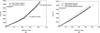Fig. 1 Relation between load and deflection of (a) a conical spring and (b) a cylindrical spring [9].

2 Analytical study

The following study was intended to highlight the impact of the geometry, the stiffness and the spatial behaviour of the end coils on the global spring. In order to do that, it is necessary to understand what happens during deflection of the spring. At the start, a cylindrical compression spring with constant pitch, not ground, and axially guided, has only a single contact point between the end coil and the floor. The axial load is, therefore, not centred on the spring but is located on its side. During the compression, this eccentric axial load causes a momentum, bending the spring until another point of the wire touches the floor. Thus, an associated contact force is created. This force evolves, as does the contact position, tending to an equilibrium state. It can be considered that, after this stabilization, the end coils have a limited impact on the remaining deflection.

2.1 Castigliano's second theorem and stiffness matrix building

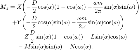
The goal of this part is to compute the global stiffness matrix of a spring element. The stiffness matrix for a curved beam element having twelve degrees of freedom was calculated by Palaninathan and Chandrasekharan [26]. The effects of axial and transverse shear forces have also been considered. However, this work has neglected the pitch of the coils, which makes the calculation easier but may well also be the source of precision mistakes. It was decided to recreate this matrix by considering the pitch of the coils. The pitch m and the helix angle α are included as shown below (see Fig. 2) and the variable ω defines the angle of the travel along the spring's primitive line, measured clockwise positive. The length of the beam is defined by ω₀, the angle subtended by the curve at the centre.

A global coordinate system and a local coordinate system are created. The first system is fixed and the second follows the primitive line with ω until the point arbitrarily called B is reached. Let A be the point at the start of the coil line, where the forces and momentum are applied. The forces represented in Figure 3 are X, Y and Z, along global axes directions. The momentum L, M and N are not represented but are on the same axes and direction as X, Y and Z, respectively.

We need now to know the internal forces and the momentums for each point on the line. First, the forces have to be transferred into the local coordinate system:$${\displaystyle \overrightarrow{F_{B,L}}}={\left\{{\left({\displaystyle \overrightarrow{F_{A,G}}}\right)}^T\times {\displaystyle \stackrel{}{Q_{GL}}}\right\}}^T$$ $$\left[\begin{array}{c}\hfill F_x\hfill \\ \hfill F_y\hfill \\ \hfill F_z\hfill \end{array}\right]={\{{\left[\begin{array}{c}\hfill X\hfill \\ \hfill Y\hfill \\ \hfill Z\hfill \end{array}\right]}^T\times \left[\begin{array}{ccc}\hfill \cos \left(\alpha \right)\cos \left(\omega \right)\hfill & \hfill \sin \left(\omega \right)\hfill & \hfill \sin \left(\alpha \right)\cos \left(\omega \right)\hfill \\ \hfill -\cos \left(\alpha \right)\sin \left(\omega \right)\hfill & \hfill \cos \left(\omega \right)\hfill & \hfill -\sin \left(\alpha \right)\sin \left(\omega \right)\hfill \\ \hfill -\sin \left(\alpha \right)\hfill & \hfill 0\hfill & \hfill \cos \left(\alpha \right)\hfill \end{array}\right]}^T.$$(2)

The matrix Q_G→L is the transfer matrix from the global to the local coordinate system. In the same way, the momentums have to be transferred but with consideration being given to the influence of the forces:$${\displaystyle \overrightarrow{M_{B,L}}}={\left\{{\left({\displaystyle \overrightarrow{M_{A,G}}}+{\displaystyle \overrightarrow{BA}}{\displaystyle \overrightarrow{F_{A,G}}}\right)}^T\times Q_{G\to L}\right\}}^T$$ $$\left[\begin{array}{c}\hfill M_x\hfill \\ \hfill M_y\hfill \\ \hfill M_z\hfill \end{array}\right]={\left\{{\left(\left[\begin{array}{c}\hfill L\hfill \\ \hfill M\hfill \\ \hfill N\hfill \end{array}\right]+\left[\begin{array}{c}\hfill -\frac{D}{2}\sin \left(\omega \right)\hfill \\ \hfill \frac{D}{2}\left(1-\cos \left(\omega \right)\right)\hfill \\ \hfill \frac{\omega m}{2\pi }\hfill \end{array}\right]\left[\begin{array}{c}\hfill X\hfill \\ \hfill Y\hfill \\ \hfill Z\hfill \end{array}\right]\right)}^T\times \left[\begin{array}{ccc}\hfill \cos \left(\alpha \right)\cos \left(\omega \right)\hfill & \hfill \sin \left(\omega \right)\hfill & \hfill \sin \left(\alpha \right)\cos \left(\omega \right)\hfill \\ \hfill -\cos \left(\alpha \right)\sin \left(\omega \right)\hfill & \hfill \cos \left(\omega \right)\hfill & \hfill -\sin \left(\alpha \right)\sin \left(\omega \right)\hfill \\ \hfill -\sin \left(\alpha \right)\hfill & \hfill 0\hfill & \hfill \cos \left(\alpha \right)\hfill \end{array}\right]\right\}}^T.$$(3)

Finally, the internal forces and the moments at B may be expressed in terms of the forces at the node A as in equations (4) $$F_x=X\cos \left(\alpha \right)\cos \left(\omega \right)-Y\cos \left(\alpha \right)\sin \left(\omega \right)-Z\sin \left(\alpha \right)$$ $$F_y=X\sin \left(\omega \right)+Y\cos \left(\omega \right)$$ $$F_x=X\sin \left(\alpha \right)\cos \left(\omega \right)-Y\sin \left(\alpha \right)\sin \left(\omega \right)+Z\cos \left(\alpha \right)$$ $$\begin{array}{l}{M}_x=X\left(\frac{D}{2}\sin \left(\alpha \right)\left(1-\cos \left(\omega \right)\right)-\frac{\omega m}{2\pi }\cos \left(\alpha \right)\text{sin}\left(\omega \right)\right)+Y\left(\frac{D}{2}\sin \left(\alpha \right)\text{sin}\left(\omega \right)-\frac{\omega m}{2\pi }\cos \left(\alpha \right)\text{cos}\left(\omega \right)\right)\\ -Z\frac{D}{2}\text{cos}\left(\alpha \right)\left(1-\cos \left(\omega \right)\right)+L\cos \left(\alpha \right)\cos \left(\omega \right)-M\cos \left(\alpha \right)\sin \left(\omega \right)-N\sin \left(\alpha \right)\end{array}$$ $$M_y=X\frac{\omega m}{2\pi }\cos \left(\omega \right)-Y\frac{\omega m}{2\pi }\sin \left(\omega \right)+Z\frac{D}{2}\text{sin}\left(\omega \right)+L\sin \left(\omega \right)+M\cos \left(\omega \right)$$ $$\begin{array}{l}{M}_z=X\left(-\frac{D}{2}\text{cos}\left(\alpha \right)\left(1-\cos \left(\omega \right)\right)-\frac{\omega m}{2\pi }\sin \left(\alpha \right)\text{sin}\left(\omega \right)\right)+Y\left(-\frac{D}{2}\cos \left(\alpha \right)\text{sin}\left(\omega \right)-\frac{\omega m}{2\pi }\text{sin}\left(\alpha \right)\text{cos}\left(\omega \right)\right)\\ -Z\frac{D}{2}\sin \left(\alpha \right)\left(1-\cos \left(\omega \right)\right)+L\sin \left(\alpha \right)\cos \left(\omega \right)-M\sin \left(\alpha \right)\sin \left(\omega \right)+N\cos \left(\alpha \right).\end{array}$$(4)

The strain energy in the beam can be expressed as:$$U_C=\frac{D}{4}{\displaystyle \underset{0}{\overset{{\omega }_0}{{\displaystyle \int }}}}\left(\frac{{\left(F_x\right)}^2}{EA}+\frac{{\left(F_y\right)}^2}{GA}+\frac{{\left(F_z\right)}^2}{GA}+\frac{{\left(M_x\right)}^2}{GJ}+\frac{{\left(M_y\right)}^2}{EI}+\frac{{\left(M_z\right)}^2}{EI}\right)d\omega$$(5)

Using Castigliano's second theorem, the deformation components can be obtained from equation (5) as:$$u_1=\frac{\delta U_C}{\delta X},u_2=\frac{\delta U_C}{\delta Y},u_3=\frac{\delta U_C}{\delta Z},u_4=\frac{\delta U_C}{\delta L},u_5=\frac{\delta U_C}{\delta M},u_6=\frac{\delta U_C}{\delta N}.$$(6)

The displacement along x, y and z global axes are respectively u₁, u₂ and u₃. The rotations along these same axes are respectively u₄, u₅ and u₆.

Using equations (4) and (5) in (6) and carrying out the indicated partial differentiation and integration, the following equation in matrix form is obtained, where the displacements are located at the point A:$$\left[\begin{array}{c}\hfill \begin{array}{c}\hfill u_1\hfill \\ \hfill u_2\hfill \\ \hfill u_3\hfill \end{array}\hfill \\ \hfill \begin{array}{c}\hfill u_4\hfill \\ \hfill u_5\hfill \\ \hfill u_6\hfill \end{array}\hfill \end{array}\right]=\left[\begin{array}{cc}\hfill \begin{array}{ccc}\hfill k_{01}\hfill & \hfill k_{07}\hfill & \hfill k_{08}\hfill \\ \hfill k_{07}\hfill & \hfill k_{02}\hfill & \hfill k_{12}\hfill \\ \hfill k_{08}\hfill & \hfill k_{12}\hfill & \hfill k_{03}\hfill \end{array}\hfill & \hfill \begin{array}{ccc}\hfill k_{09}\hfill & \hfill k_{10}\hfill & \hfill k_{11}\hfill \\ \hfill k_{13}\hfill & \hfill k_{14}\hfill & \hfill k_{15}\hfill \\ \hfill k_{16}\hfill & \hfill k_{17}\hfill & \hfill k_{18}\hfill \end{array}\hfill \\ \hfill \begin{array}{ccc}\hfill k_{09}\hfill & \hfill k_{13}\hfill & \hfill k_{16}\hfill \\ \hfill k_{10}\hfill & \hfill k_{14}\hfill & \hfill k_{17}\hfill \\ \hfill k_{11}\hfill & \hfill k_{15}\hfill & \hfill k_{18}\hfill \end{array}\hfill & \hfill \begin{array}{ccc}\hfill k_{04}\hfill & \hfill k_{19}\hfill & \hfill k_{20}\hfill \\ \hfill k_{19}\hfill & \hfill k_{05}\hfill & \hfill k_{21}\hfill \\ \hfill k_{20}\hfill & \hfill k_{21}\hfill & \hfill k_{06}\hfill \end{array}\hfill \end{array}\right]\left[\begin{array}{c}\hfill \begin{array}{c}\hfill X\hfill \\ \hfill Y\hfill \\ \hfill Z\hfill \end{array}\hfill \\ \hfill \begin{array}{c}\hfill L\hfill \\ \hfill M\hfill \\ \hfill N\hfill \end{array}\hfill \end{array}\right]$$ $$U_i=M_{F_{ii}}.F_i.$$(7)

It can be observed that the matrix is symmetrical. The detailed equations are available in Appendix A. Now, the 6 × 6 stiffness matrix can be created, based on the flexibility one already made.$$M_{K_{ii}}=M_{F_{ii}}^{-1}.$$(8)

To build the stiffness of the whole element, we create a transfer matrix T_i→j based on a hypothesis of small displacements. It represents the impact of the displacements or loads of one extremity on the other:

And we have: $$T_{i\to j}=\left[\begin{array}{cc}\hfill \begin{array}{ccc}\hfill \begin{array}{c}\hfill \begin{array}{c}\hfill -1\hfill \\ \hfill 0\hfill \\ \hfill 0\hfill \end{array}\hfill \\ \hfill \begin{array}{c}\hfill 0\hfill \\ \hfill 0\hfill \\ \hfill 0\hfill \end{array}\hfill \end{array}\hfill & \hfill \begin{array}{c}\hfill \begin{array}{c}\hfill 0\hfill \\ \hfill -1\hfill \\ \hfill 0\hfill \end{array}\hfill \\ \hfill \begin{array}{c}\hfill 0\hfill \\ \hfill 0\hfill \\ \hfill 0\hfill \end{array}\hfill \end{array}\hfill & \hfill \begin{array}{c}\hfill \begin{array}{c}\hfill 0\hfill \\ \hfill 0\hfill \\ \hfill -1\hfill \end{array}\hfill \\ \hfill \begin{array}{c}\hfill 0\hfill \\ \hfill 0\hfill \\ \hfill 0\hfill \end{array}\hfill \end{array}\hfill \end{array}\hfill & \hfill \begin{array}{ccc}\hfill \begin{array}{c}\hfill \begin{array}{c}\hfill 0\hfill \\ \hfill \omega m/2\pi \hfill \\ \hfill -D(1-\cos \left(\omega \right))/2\hfill \end{array}\hfill \\ \hfill \begin{array}{c}\hfill --1\hfill \\ \hfill 0\hfill \\ \hfill 0\hfill \end{array}\hfill \end{array}\hfill & \hfill \begin{array}{c}\hfill \begin{array}{c}\hfill -\omega m/2\pi \hfill \\ \hfill 0\hfill \\ \hfill -D\sin \left(\omega \right)/2\hfill \end{array}\hfill \\ \hfill \begin{array}{c}\hfill 0\hfill \\ \hfill -1\hfill \\ \hfill 0\hfill \end{array}\hfill \end{array}\hfill & \hfill \begin{array}{c}\hfill \begin{array}{c}\hfill D(1-\cos \left(\omega \right))/2\hfill \\ \hfill D\sin \left(\omega \right)/2\hfill \\ \hfill 0\hfill \end{array}\hfill \\ \hfill \begin{array}{c}\hfill 0\hfill \\ \hfill 0\hfill \\ \hfill -1\hfill \end{array}\hfill \end{array}\hfill \end{array}\hfill \end{array}\right]$$(9) $$M_{K_{ij}}=M_{K_{ii}}.T_{i\to j}$$(10) $$M_{K_{ji}}=T_{i\to j}^T.M_{K_{ii}}=M_{K_{ij}}^T$$(11) $$M_{K_{jj}}=T_{i\to j}^T.M_{K_{ij}}.$$(12)

We can build the local stiffness matrix of our element:$$M_{K_{ele{m}_L}}=\left[\begin{array}{cc}\hfill M_{K_{ii}}\hfill & \hfill M_{K_{ij}}\hfill \\ \hfill M_{K_{ji}}\hfill & \hfill M_{K_{jj}}\hfill \end{array}\right].$$(13)

To check the accuracy of the matrix, a finite element model was made on Abaqus. It was designed by placing data points and by connecting them with a spline. This spline allowed the exact shape of the spring's mean wire to be well approximated without having to compute a large amount of points (see Fig. 4). Several tests were performed with whole and non-whole numbers of coils. The average error between the models was around 1% which confirms the accuracy of this matrix.

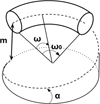Fig. 2 Curved beam characteristics.

Fig. 3 Curved beam coordinate force system.

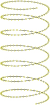Fig. 4 Abaqus geometry of the spring.

2.2 Geometrical calculation of the contact points

Geometrical calculation was used to determine where the spring touched the floor at a point other than the one where the force is applied. In order to set the boundary conditions of the model, it is necessary to know the positions of its particular points. The following calculation considers the end coil as a rigid body, which is a good approximation because it is slightly deformed. We create a curved line for the last coil of the spring and a plane. To simplify the equations, let us consider that it is the plane, not the coil, that is inclined. We have a curved line with a pitch m_e and a diameter D and a plane in rotation around the y axis, displaced from the z axis by D/2, inclined by θ (see Fig. 5). The origin for both the cylindrical and Cartesian coordinate systems is in the centre of the coil, on the floor.

The coil expression in cylindrical coordinates is defined by:$$r=\frac{D}{2}\text{and}{z}_c=\frac{\omega m_e}{2\pi }.$$(14)

The plane expression can be written in Cartesian coordinates as:$$z_p=\left(\frac{D}{2}-x\right)\tan \left(\theta \right).$$(15)

In order to compare them, the plane of coordinate system has to be changed. In cylindrical coordinates, the vertical expression for the planes becomes:$$z_p=\frac{D}{2}\text{tan}\left(\theta \right)\left(1-\cos \left(\omega \right)\right).$$(16)

Now we have the two expressions in the same coordinate system, giving two curves. At the contact point, the curves have to touch and also be tangent to each other. So, we have contact when:$$z_p=z_c\text{and}{z^{\prime }}_p={z^{\prime }}_c$$(17)with:$${z^{\prime }}_c=\frac{m_e}{2\pi }\text{and}{z^{\prime }}_p=\frac{D}{2}\tan \left(\theta \right)\text{sin}\left(\omega \right).$$(18)

Now, if p is the percentage of this coil, we have ω=p2π. From equations (14), (16), (17) and (18) we can compute:$$p2\pi \frac{m_e}{2\pi }-\frac{D}{2}\tan \left(\theta \right)\left(1-\cos \left(p2\pi \right)\right)=0$$ $$\frac{m_e}{2\pi }-\frac{D}{2}\tan \left(\theta \right)\sin \left(p2\pi \right)=0$$ $$\text{So}:p-\frac{1-\cos \left(p2\pi \right)}{2\pi \sin \left(p2\pi \right)}=0.$$(19)

We obtain a solvable equation with p (Eq. (19)). Note that this equation does not depend on original input data like the pitch or the diameter of the coil. We can conclude this point is a common value for all the coils (with a constant pitch) and p = 0.371 = 37.1%. For this kind of coil, this value can be understood in two ways: the contact is made at 37.1% of the pitch starting at the floor or at 37.1% of the angle of the coil, starting at the floor (see Fig. 6). The second phase of the curve occurs during the stabilisation of the end coils. We now know that the end coils bend until the point at p reaches the floor. But we suppose that there is another transition during the deflection. The end coil has to tend toward an equilibrium state where the second application point becomes at the radial position opposite of the point where the force is applied. From this state, the end coil no longer moves and it can be frozen during the third phase and until the end of compression. This stabilisation point is geometrically positioned at 50% of the end coil.

This was later confirmed by numerical tests on Abaqus. Two supports that managed contact with the wire, set boundary conditions and connectors between the wires and forced displacement of the upper support were modelled (see Fig. 7). The number of meshes on the end coils was high, with close to 200 elements. Figure 8 shows the contact force distribution during the compression and its position along the end coil. The left red curve at 0%, the start of the coil, is where the force is applied. The right blue curve represents the second point of contact. The first contact clearly appears close to 35%, then slides along the coil until it reaches approximately 50% of it. The slight difference comes from our hypothesis of y axis rotation only and our rigid body hypothesis but it can be assumed as negligible because of the small height difference between two points situated 2% of the coil away from each other. For all the springs modelled, the first contact point appeared between 33 and 39% and travelled until a stabilised point was reached between 48 and 51%.

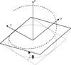Fig. 5 End coil's mean line and inclined plane.

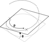Fig. 6 Curved beam contact point.

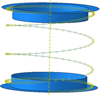Fig. 7 Complete Abaqus #4 model.

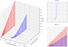Fig. 8 Abaqus results on contact reaction forces for spring #4.

2.3 Global spring stiffness building

Once the points of interest were known, it is necessary to partition the spring. In order to reach data from points located at 0.371 (points B and G) and 0.500 (points C and F) on the end coils, several partitions are needed, leading to a total of seven elements (see Fig. 9). Each of them includes its diameters D and d, its pitch m (therefore its helix angle α) and its angular length ω₀.

To include all the elements in a global system, it is necessary to rotate the local element stiffness matrixes by the sum of the angular length ω₀ of the coils above it. The starting element is at the top, where the forces are applied.$${\omega }_{r1}=0$$ $${\omega }_{rn}={\omega }_{rn-1}+{\omega }_{0n-1}$$ $$q_{G\to L}=\left[\begin{array}{ccc}\hfill \cos {\omega }_r\hfill & \hfill \sin {\omega }_r\hfill & \hfill 0\hfill \\ \hfill -\sin {\omega }_r\hfill & \hfill \cos {\omega }_r\hfill & \hfill 0\hfill \\ \hfill 0\hfill & \hfill 0\hfill & \hfill 1\hfill \end{array}\right]$$ $$Q_{G\to L}=\left[\begin{array}{cc}\hfill \begin{array}{cc}\hfill q_{G\to L}\hfill & \hfill 0_{\mathrm{3,3}}\hfill \\ \hfill 0_{\mathrm{3,3}}\hfill & \hfill q_{G\to L}\hfill \end{array}\hfill & \hfill \begin{array}{cc}\hfill 0_{\mathrm{3,3}}\hfill & \hfill 0_{\mathrm{3,3}}\hfill \\ \hfill 0_{\mathrm{3,3}}\hfill & \hfill 0_{\mathrm{3,3}}\hfill \end{array}\hfill \\ \hfill \begin{array}{cc}\hfill 0_{\mathrm{3,3}}\hfill & \hfill 0_{\mathrm{3,3}}\hfill \\ \hfill 0_{\mathrm{3,3}}\hfill & \hfill 0_{\mathrm{3,3}}\hfill \end{array}\hfill & \hfill \begin{array}{cc}\hfill q_{G\to L}\hfill & \hfill 0_{\mathrm{3,3}}\hfill \\ \hfill 0_{\mathrm{3,3}}\hfill & \hfill q_{G\to L}\hfill \end{array}\hfill \end{array}\right]$$ $$M_{K_{ele{m}_G}}=Q_{G\to L}.M_{K_{ele{m}_L}}.{Q_{G\to L}}^T=\left[\begin{array}{cc}\hfill M_{ele{m}_{ii}}\hfill & \hfill M_{ele{m}_{ij}}\hfill \\ \hfill M_{ele{m}_{ji}}\hfill & \hfill M_{ele{m}_{jj}}\hfill \end{array}\right].$$(20)

The spring stiffness matrix can now be built in the global system with all seven elements: $$M_K=\left[\begin{array}{cccccc}\hfill M_{1_{ii}}\hfill & \hfill M_{1_{ij}}\hfill & \hfill 0\hfill & \hfill \cdots \hfill & \hfill 0\hfill & \hfill 0\hfill \\ \hfill M_{1_{ji}}\hfill & \hfill M_{1_{ij}}+M_{2_{ii}}\hfill & \hfill M_{2_{ij}}\hfill & \hfill \cdots \hfill & \hfill 0\hfill & \hfill 0\hfill \\ \hfill 0\hfill & \hfill M_{2_{ji}}\hfill & \hfill M_{2_{jj}}+M_{3_{ii}}\hfill & \hfill \cdots \hfill & \hfill 0\hfill & \hfill 0\hfill \\ \hfill ⋮\hfill & \hfill ⋮\hfill & \hfill ⋮\hfill & \hfill \ddots \hfill & \hfill ⋮\hfill & \hfill ⋮\hfill \\ \hfill 0\hfill & \hfill 0\hfill & \hfill 0\hfill & \hfill \cdots \hfill & \hfill M_{6_{jj}}+M_{7_{ii}}\hfill & \hfill M_{7_{ij}}\hfill \\ \hfill 0\hfill & \hfill 0\hfill & \hfill 0\hfill & \hfill \cdots \hfill & \hfill M_{7_{ji}}\hfill & \hfill M_{7_{jj}}\hfill \end{array}\right]$$(21) $$F=M_K.U.$$(22)

With the global stiffness matrix built, the degrees of freedom have to be set. For all the 8 points, 6 degrees of freedom have to be assigned for each of the 3 phases. For each of them, either it is known to be free, so the displacement is unknown and the external force is null, or we set the displacement and the force linked to it is unknown. So, for each row, either the value of F, or the value of U is known. All set values are available in Appendix B. Because this model is created with 7 elements, this involves solving 48 equations with 48 unknown values for each phase. To dissociate the unknown and the known values, we use:$$0_{\mathrm{48,1}}=M_K.U-I_{48}.F$$(23) $$0_{\mathrm{48,1}}=A.X-b.$$(24)

The vector b is the sum of the products between the known values and their associated matrix column (M_K for displacement and −I₄₈ for loads). Matrix A is the concatenation of the associated matrix column of the unknown values. Both have to be structured in the same order: the first row corresponds to the x behaviour (displacement or force) of point A, the second row to the y behaviour to the same point, and so on. The vector X is the storage vector of all unknown values, it is what needs to be calculated. Therefore:$$X=A^{-1}.b.$$(25)

By solving X for each phase, we can calculate the stiffness of the spring during the whole deflection. We obtain a tri-linear curve with only six input parameters: the spring diameter D, the wire diameter d, the Young's modulus E, the shear modulus G, the number of active coils n_a, the active pitch m_a.

Moreover, end coils (one turn at each side) are commonly designed with an axial pitch equal to the wire diameter. Such a design induces a sudden change in the spring pitch at the end of the end coil when passing from d to the pitch of the active coils as can been seen in Figure 10 left. Unfortunately, manufacturers cannot make this angular geometry. The pitch must evolve smoothly and therefore the initial pitch must be lower. To precisely model the end coils a seventh parameter has been implemented for the first time in this analytical model: the helix angle coefficient of end coils f. It represents the design geometry ratio between the real pitch of end coils and the common one (d). Figure 10 presents the evolution of the height (z) as a function of the angle of the travel along the spring's primitive line (ω) for several values of f. For “classic” spring geometry, f ≈ 0.7. In our study, some of the springs had end coils where the points C and F were already in contact with the floor. In this case, the helix angle coefficient f ≈ 0 and only the third phase exists.

This f ratio is applied to the heights of points B, C, F and G. It has a non-negligible impact on the curve, pushing the third phase forward by modifying stiffnesses and the necessary deflection to obtain contacts. These phenomena strengthen our idea that end coils must no longer be neglected. Both their stiffness and their geometry have to be considered during dimensioning and designing phases.

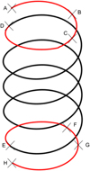Fig. 9 Spring partitions.

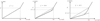Fig. 10 Impact of helix angle ratio on geometry.

3 Comparison with experimental data

To verify our model, it was confronted with experimental values. The method consisted of measuring all the dimensions of the springs precisely, evaluating the elastic and torsion moduli and then computing the new analytical model curve. Even though the springs had no risk of buckling, it was desirable to avoid any misplacement for the compression start, so the experimental tests were carried out with an axial guide.

Each experiment included three springs and each spring was measured several times. The value of f was estimated from the geometry of the end coils (see Tab. 1).

All the springs were made from the same wire (which is why d was always 1.8mm). Thus, they were all known to share the same material characteristics. In order to accurately estimate E and G, it was decided to take the biggest spring available, which had no bilinearity, so the analytical curve could be adjusted (see Fig. 11i). We found E = 180000 MPa and G = 73500 MPa.

All the input data being known, it was possible to create all the curves. Among them (see Fig. 11), the springs with small index (D/d ratio) and small number of active coils showed the greatest imprecision of the classic formula. For springs with large dimensions, the impact of the end coils was almost negligible but for smaller ones, there were as many end coils as active coils. Ignoring them would mean ignoring half of the spring.

Figures 11a, 11b, 11d compare the experimental and analytical curves of springs #1, #2 and #4. Predictions by the classic formula are far from the behaviour of these real springs, even though they are still in the validity range of the formula [6,28]. The new analytical model is superimposed on the experimental data. It finds very good stiffnesses and accurate transition points.

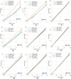Fig. 11 Analytical and experimental load-deflection curves.

4 Discussion

The aim of this study was to propose a new approach to cylindrical compression springs with constant pitch, not ground by performing analytical, finite-element and experimental analyses. In this case, the force-length relationship was governed by a linear equation. It appeared that this formula did not predict the springs' behaviour with enough accuracy. The experimental study clearly showed the non-linear behaviour of springs with a small number of active coils and small index (ratio of mean diameter/wire diameter). Numerical simulations highlighted that the initial rate of the spring was due to the disequilibrium of loads in the end coils. For the first time, an analytical model now enables the initial behaviour of compression springs to be defined precisely. This was achieved using Castigliano's second theorem on curved beam elements and considering the helix angle, the geometry of the end coils, the in-plane and normal-to-plane forces, the spring's manufacturing imperfections and the non-parallel ends.

The results given by this tri-linear model were successfully confronted with experimental data. The model gave more accurate results for all spring dimensions but, in particular, for compression springs with a small number of active coils. This model was also compared with the numerical Abaqus wire model. The average stiffness error between the two was around 0.5%. Even if we consider that both models give the same results, this new analytical one compute instantly where numerical programs take around 20 min to calculate (if just the “job” calculation time is considered, without the time needed to design the geometry of the object and the time needed to exploit the results).

This tool can simplify the dimensioning phase by saving a lot of computing time and will be useful for researchers seeking to perform optimisation as in [29,30] with compression springs. In domains where high precision is required, the accuracy level of the model can enable researchers to understand the behaviour of the springs with more exactitude and provide more efficient systems [3]. It can be opportunely exploited to enlarge the common operating and validity ranges of compression springs, which currently appears to be very restrictive [6,28]. Finally, it can assist manufacturers in the design phases to predict the actual free length needed in order to accurately reach the loads theoretically specified for given lengths [5].

This work may be continued to upgrade future spring calculation. The evaluation of forces can be used to calculate all stresses everywhere along the wire. Also, the stiffness element matrix calculated in Section 2.1 can be used for extension and torsion springs.

However, the model can still be improved. For example, all experimental springs have numbers of active coils that are close to integers. More tests have to be done to confirm whether the model is still accurate with more random numbers of active coils. We can imagine recreating this model by considering an eventual misplacement of the spring during the initial compression. Moreover, the model does not yet consider the final compression behaviour of the spring, when it approaches its solid length. We can imagine adding a fourth phase to include this.

Appendix A Local flexibility matrix elements calculation

$$i_1={\omega }_0$$ $$i_s=1-\cos {\omega }_0$$ $$i_c=\sin {\omega }_0$$ $$i_{ss}=\frac{{\omega }_0}{2}-\frac{\sin 2{\omega }_0}{4}$$ $$i_{cc}=\frac{{\omega }_0}{2}+\frac{\sin 2{\omega }_0}{4}$$ $$i_{cs}=\frac{1}{2}-\frac{{\cos }^2{\omega }_0}{2}$$ $$i_{xs}=\sin {\omega }_0-{\omega }_0\cos {\omega }_0$$ $$i_{xc}={\omega }_0\sin {\omega }_0+\cos {\omega }_0-1$$ $$i_{xcs}=\frac{\sin 2{\omega }_0-2{\omega }_0\cos 2{\omega }_0}{8}$$ $$i_{xss}=\frac{2{\omega }_0\left({\omega }_0-\sin 2{\omega }_0\right)-\cos 2{\omega }_0+1}{8}$$ $$i_{xcc}=\frac{2{\omega }_0\left({\omega }_0+\sin 2{\omega }_0\right)+\cos 2{\omega }_0-1}{8}$$ $$i_{xxss}=\frac{4{\omega }_0^3+\left(3-6{\omega }_0^2\right)\sin 2{\omega }_0-6{\omega }_0\cos 2{\omega }_0}{24}$$ $$i_{xxcc}=\frac{4{\omega }_0^3-\left(3-6{\omega }_0^2\right)\sin 2{\omega }_0+6{\omega }_0\cos 2{\omega }_0}{24}$$ $$i_{xxcs}=\frac{\left(1-2{\omega }_0^2\right)\cos 2{\omega }_0+2{\omega }_0\sin 2{\omega }_0-1}{8}$$ $$i_{1c}={\omega }_0-\sin {\omega }_0$$ $$i_{1c2}=\frac{6{\omega }_0+\sin 2{\omega }_0-8\sin {\omega }_0}{4}$$ $$i_{xs1c}=\frac{8\sin {\omega }_0-\sin 2{\omega }_0+2{\omega }_0\cos 2{\omega }_0-8{\omega }_0\cos {\omega }_0}{8}$$ $$i_{xc1c}=-\frac{2{\omega }_0\left({\omega }_0+\sin 2{\omega }_0-4\sin {\omega }_0\right)+\cos 2{\omega }_0-8\cos {\omega }_0+7}{8}$$ $$i_{s1c}=\frac{1-\cos {\omega }_0\left(2-\cos {\omega }_0\right)}{2}$$ $$i_{c1c}=\frac{4\sin {\omega }_0-2{\omega }_0-\sin 2{\omega }_0}{4}$$ $$C={\cos }^2\alpha$$ $$S={\sin }^2\alpha$$ $$Q=\sin \alpha \cos \alpha$$ $$I=\frac{\pi d^4}{64}$$ $$J=\frac{\pi d^4}{32}$$ $$A=\frac{\pi d^2}{4}$$ $$k_{01}=\frac{i_{cc}DC}{2EA}+\frac{D{i}_{ss}+i_{cc}\text{DS}}{2GA}+\frac{\frac{D^3}{4}{i}_{1c2}S+i_{xxss}C\frac{D{m}^2}{4{\pi }^2}-i_{xs1c}\frac{D^{2}m}{2\pi }Q}{2GJ}+\frac{i_{xxcc}\frac{D{m}^2}{4{\pi }^2}+i_{1c2}\frac{D^3}{4}C+i_{xxss}S\frac{D{m}^2}{4{\pi }^2}+i_{xs1c}\frac{D^{2}m}{2\pi }Q}{2EI}$$ $$k_{02}=\frac{i_{ss}DC}{2EA}+\frac{i_{cc}D+i_{ss}\text{DS}}{2GA}+\frac{\frac{D^3}{4}{i}_{ss}\text{S}+i_{xxcc}C\frac{D{m}^2}{4{\pi }^2}-i_{xcs}\frac{D^{2}m}{2\pi }Q}{2GJ}+\frac{i_{xxss}\frac{D{m}^2}{4{\pi }^2}+i_{ss}\frac{D^3}{4}C+i_{xxcc}S\frac{D{m}^2}{4{\pi }^2}+i_{xcs}\frac{D^{2}m}{2\pi }Q}{2EI}$$ $$k_{03}=\frac{i_{1}DS}{2EA}+\frac{i_1\text{DC}}{2GA}+\frac{i_{1c2}\frac{D^3}{4}C}{2GJ}+\frac{\left(i_{ss}+i_{1c2}S\right)\frac{D^3}{4}}{2EI}$$ $$k_{04}=\frac{i_{cc}\text{D}C}{2GJ}+\frac{i_{ss}D+i_{cc}DS}{2EI}$$ $$k_{05}=\frac{D{i}_{ss}C}{2GJ}+\frac{i_{cc}D+i_{ss}DS}{2EI}$$ $$k_{06}=\frac{i_{1}DS}{2GJ}+\frac{i_{1}DC}{2EI}$$ $$k_{07}=\frac{-D{i}_{cs}C}{2EA}+\frac{D{i}_{cs}C}{2GA}+\frac{\frac{D^3}{4}{i}_{s1c}S+i_{xxcs}C\frac{D{m}^2}{4{\pi }^2}-\left(i_{xss}+i_{xc1c}\right)\frac{D^{2}m}{4\pi }Q}{2GJ}+\frac{\frac{D^3}{4}{i}_{s1c}C-i_{xxcs}C\frac{D{m}^2}{4{\pi }^2}+\left(i_{xss}+i_{xc1c}\right)\frac{D^{2}m}{4\pi }Q}{2EI}$$ $$k_{08}=\frac{-D{i}_{c}Q}{2EA}+\frac{D{i}_{c}Q}{2GA}+\frac{i_{xs1c}\frac{D^{2}m}{4\pi }C-\frac{D^3}{4}{i}_{1c2}Q}{2GJ}+\frac{\frac{D^3}{4}{i}_{1c2}Q+\left(i_{xs1c}S+i_{xcs}\right)\frac{D^{2}m}{4\pi }}{2EI}$$ $$k_{09}=\frac{i_{c1c}{\text{D}}^{2}Q-i_{xcs}\frac{Dm}{\pi }C}{4GJ}-\frac{i_{c1c}{\text{D}}^{2}Q-i_{xcs}\frac{Dm}{\pi }C}{4EI}$$ $$k_{10}=\frac{i_{xss}\frac{Dm}{\pi }C-i_{s1c}{\text{D}}^{2}Q}{4GJ}+\frac{i_{s1c}{\text{D}}^{2}Q+i_{xss}\frac{Dm}{\pi }S+i_{xcc}\frac{Dm}{\pi }}{4EI}$$ $$k_{11}=\frac{i_{xs}\frac{Dm}{\pi }Q-i_{1c}{\text{D}}^{2}S}{4GJ}-\frac{i_{1c}{\text{D}}^{2}C+i_{xs}\frac{Dm}{\pi }Q}{4EI}$$ $$k_{12}=\frac{D{i}_{s}Q}{2EA}-\frac{D{i}_{s}Q}{2GA}+\frac{i_{xc1c}\frac{D^{2}m}{4\pi }C-\frac{D^3}{4}{i}_{s1c}Q}{2GJ}+\frac{\frac{D^3}{4}{i}_{s1c}Q+\left(i_{xc1c}S-i_{xss}\right)\frac{D^{2}m}{4\pi }}{2EI}$$ $$k_{13}=\frac{i_{cs}{\text{D}}^{2}Q-i_{xcc}\frac{Dm}{\pi }C}{4GJ}-\frac{i_{cs}{\text{D}}^{2}Q+\frac{Dm}{\pi }\left(i_{xcc}S+i_{xss}\right)}{4EI}$$ $$k_{14}=\frac{i_{xcs}\frac{Dm}{\pi }C-i_{ss}{\text{D}}^{2}Q}{4GJ}+\frac{i_{ss}{\text{D}}^{2}Q-i_{xcs}\frac{Dm}{\pi }C}{4EI}$$ $$k_{15}=\frac{-i_s{\text{D}}^{2}S+i_{xc}\frac{Dm}{\pi }Q}{4GJ}-\frac{i_s{\text{D}}^{2}C+i_{xc}\frac{Dm}{\pi }Q}{4EI}$$ $$k_{16}=\frac{{\text{D}}^2\left(i_{ss}-i_{c1c}S\right)}{4EI}-\frac{i_{c1c}{\text{D}}^{2}C}{4GJ}$$ $$k_{17}=\frac{i_{s1c}{\text{D}}^{2}C}{4GJ}+\frac{{\text{D}}^2\left(i_{cs}+i_{s1c}S\right)}{4EI}$$ $$k_{18}=\frac{i_{1c}{\text{D}}^{2}Q}{4GJ}-\frac{i_{1c}{\text{D}}^{2}Q}{4EI}$$ $$k_{19}=\frac{D{i}_{cs}C}{2EI}-\frac{D{i}_{cs}C}{2GJ}$$ $$k_{20}=\frac{i_{c}DQ}{2EI}-\frac{i_c\text{D}Q}{2GJ}$$ $$k_{21}=\frac{D{i}_{s}Q}{2GJ}-\frac{D{i}_{s}Q}{2EI}$$

Appendix B

References

All Tables

All Figures

	Fig. 1 Relation between load and deflection of (a) a conical spring and (b) a cylindrical spring [9].
In the text

	Fig. 2 Curved beam characteristics.
In the text

	Fig. 3 Curved beam coordinate force system.
In the text

	Fig. 4 Abaqus geometry of the spring.
In the text

	Fig. 5 End coil's mean line and inclined plane.
In the text

	Fig. 6 Curved beam contact point.
In the text

	Fig. 7 Complete Abaqus #4 model.
In the text

	Fig. 8 Abaqus results on contact reaction forces for spring #4.
In the text

	Fig. 9 Spring partitions.
In the text

	Fig. 10 Impact of helix angle ratio on geometry.
In the text

	Fig. 11 Analytical and experimental load-deflection curves.
In the text

References

- N. Gubeljak, V. Vejborný, Mechanical springs, Maribor University, https://www.academia.edu/23350011/Mechanical_Springs [Google Scholar]
- S.S. Gaikwad, P.S. Kachare, Static analysis of helical compression spring used in two-wheeler horn, IJEAT 2, 161–165 (2013) [Google Scholar]
- S.P. Laksono, Investigation of wire diameter of helical compression spring for payload separation, Jurnal Teknologi Dirgantara 19, 15–24 (2021) [Google Scholar]
- M. Paredes, Enhanced formulae for determining both free length and rate of cylindrical compression springs, ASME J. Mech. Des. 138, 021404 (2016) [CrossRef] [Google Scholar]
- Spring Calculator software from Institute of Spring Technology, https://www.ist.org.uk [Google Scholar]
- Norme NF EN 13906-1, Ressorts hélicoïdaux cylindriques fabriqués à partir de fils ronds et de barres, Calcul et conception, Partie 1 : Ressorts de compression, AFNOR (2002) [Google Scholar]
- P.S. Valsange, Design of helical coil compression spring: a review, Int. J. Eng. Res Appl. 2, 513–522 (2012) [Google Scholar]
- Spring-I-pedia, http://springipedia.com/extension-designtheory.asp [Google Scholar]
- D. Siddharth Yadav, S. Lata, Design development and analysis of cylindrical spring with variable pitch for two wheelers, in: A. Sharma, R. Singh (Eds.), Materials Todays: Proceedings 47(11), 3rd International Conference on Advances in Mechanical Engineering and Nanotechnology, Elsevier, 2021, pp. 3105–7853 [Google Scholar]
- S. Pattar, S.J. Sanjay, V.B. Math, Static analysis of helical compression spring, Int. J. Res. Eng. Technol. 03, 835–838 (2014) [CrossRef] [Google Scholar]
- M. Shimoseki, T. Hamano, T. Imaizumi, FEM for Springs, Berlin, Heidelberg, 2003 2003 [CrossRef] [Google Scholar]
- R.R.D. Ananto, Andoko, Coil spring type analysis using the finite element method, IOP Conf. Series: Mater. Sci. Eng. 1034, 012016 (2021) [CrossRef] [Google Scholar]
- B. Gironnet, G. Louradour, Comportement dynamique des ressorts, Techniques de l'Ingénieur BD2, B610-1-B610-11 (1983) [Google Scholar]
- V. Bhatt, P. Rawat, D. Kumar, Finite element analysis-modelling and simulation of coil springs, Juni Khyat 10, 127–136 (2020) [Google Scholar]
- F. De Crescenzo, P. Salvini, Influence of coil contact on static behavior of helical compression springs, IOP Conf. Ser.: Mater. Sci. Eng. 1038, 012064 (2021) [CrossRef] [Google Scholar]
- D. Fakhreddine, T. Mohamed, A. Said, D. Abderrazek, H. Mohamed, Finite element method for the stress analysis of isotropic cylindrical helical spring, Eur. J. Mech. A: Solids 24, 1068–1078 (2005) [CrossRef] [Google Scholar]
- A.Y. Babenko, B. Soltannia, P.S. Mobarakeh, Solving geometrically nonlinear problem on deformation of a helical spring through variational methods, Int. J. Mech. Appl. 8, 21–24 (2018) [Google Scholar]
- Z. Gu, X. Hou, J. Ye, Design and analysis method of nonlinear helical springs using a combining technique: finite element analysis, constrained latin hypercube sampling and genetic programming, J. Mech. Eng. Sci. 1–14 (2021) [Google Scholar]
- D. Qiu, S. Seguy, M. Paredes, Design of cubic stiffness for the absorber of nonlinear energy sink (NES), in: XXth Symposium Vibrations, Shocks and Noise VISHNO, 2295–2300 (2016) [Google Scholar]
- E. Rodriguez, Étude du comportement des ressorts coniques et ressorts de torsion en vue du développement d'outils de synthèse associés, PhD thesis, INSA de Toulouse, 2006 http://www.theses.fr/2006ISAT0032 [Google Scholar]
- E. Rodriguez, M. Paredes, M. Sartor, Analytical behaviour law for a constant pitch conical compression spring, ASME J. Mech. Des. 129, 1352–1356 (2006) [CrossRef] [Google Scholar]
- M. Paredes, T. Stephan, H. Orcière, Enhanced formulae for determining the axial behaviour of cylindrical extension springs, Mech. Ind. 20, 625 (2019) [CrossRef] [EDP Sciences] [Google Scholar]
- P.C. Tse, C.T. Lung, Large deflections of elastic composite circular springs under uniaxial tension, Int. J. Non-Linear Mech. 35, 293–307 (2000) [CrossRef] [Google Scholar]
- S. Ayadi, E. Hadj-Taieb, Influence des caractéristiques mécaniques sur la propagation des ondes de deformations linéaires dans les ressorts hélicoidaux, Mech. Ind. 7, 551–563 (2006) [Google Scholar]
- A. Hamza, S. Ayadi, E. Hadj-Taieb, Resonance phenomenon of strain waves in helical compression springs, Mech. Ind. 14, 253–265 (2013) [CrossRef] [EDP Sciences] [Google Scholar]
- R. Palaninathan, P.S. Chandrasekharan, Curved beam element stiffness matrix formulation, Comput. Struct. 21, 663–669 (1985) [CrossRef] [Google Scholar]
- C. Dym, Consistent derivations of spring rates for helical springs, ASME J. Mech. Des. 131 (2009) [Google Scholar]
- DIN 2088, DIN 2089-1, DIN 2089-2, Burggrafenstraße 6, postfach 11 07, 10787 Berlin, Germany [Google Scholar]
- O. Braydi, C. Gogu, M. Paredes, Robustness and reliability investigations on a nonlinear energy sink device concept, Mech. Ind. 21, 603 (2020) [CrossRef] [EDP Sciences] [Google Scholar]
- M. Paredes, Développement d'outils d'assistance à la conception optimale des liaisons élastiques par ressorts, PhD thesis, INSA de Toulouse (2000) [Google Scholar]
Cite this article as: G. Cadet, M. Paredes, H. Orcière, Improved analytical model for cylindrical compression springs not ground considering end behavior of end coils, Mechanics & Industry 22, 50 (2021)