| Issue |
Mechanics & Industry
Volume 23, 2022
|
|
|---|---|---|
| Article Number | 1 | |
| Number of page(s) | 8 | |
| DOI | https://doi.org/10.1051/meca/2021052 | |
| Published online | 20 January 2022 | |
Regular Article
An indicator of porosity through simulation of melt pool volume in aluminum wire arc additive manufacturing
1
Univ. Grenoble Alpes, CNRS, Grenoble INP, G-SCOP, 38000 Grenoble, France
2
S.mart Grenoble Alpes, 38000 Grenoble, France
* e-mail: This email address is being protected from spambots. You need JavaScript enabled to view it.
Received:
15
September
2021
Accepted:
30
December
2021
Abstract
Managing the quality of functional parts is a key challenge in wire arc additive manufacturing. In case of additive production of aluminum parts, porosity is one of the main limitations of this process. This paper provides an indicator of porosity through the simulation of melt pool volume in aluminum wire arc additive manufacturing. First, a review of porosity formation during WAAM process is presented. This review leads to the proposal of this article: monitoring the porosity inside produced part can be achieved through the melt pool volume monitoring. An adapted Finite Element model is then proposed to determine the evolution of the melt pool volume throughout the manufacturing process of the part. This model is validated by experimental temperature measurement. Then, in order to study the link between the porosity and the melt pool volume, two test parts are chosen to access to two different pore distributions. These two parts are simulated and produced. The porosity rates of produced parts are then measured by X-ray tomography and compared to the simulated melt pool volumes. The analysis of the results highlights the interest of the melt pool volume as a predictive indicator of the porosity rate.
Key words: Additive manufacturing / wire arc additive manufacturing / quality / porosity / process simulation
© N. Béraud et al., Published by EDP Sciences 2022
 This is an Open Access article distributed under the terms of the Creative Commons Attribution License (https://creativecommons.org/licenses/by/4.0), which permits unrestricted use, distribution, and reproduction in any medium, provided the original work is properly cited.
1 Introduction
Wire arc additive manufacturing (WAAM) is an additive manufacturing process that enables the production of parts from a metallic wire and the use of arc welding technology as heat source [1]. Some benefits can explain the interest from industrial and research community [2]. Among them, WAAM technology is able to offer high deposition rates and large parts production in a wide range of materials. Its adoption is likewise facilitated by the low cost of the production machine and the security framework provided by the usage of wire instead of powder [3].
Managing the quality of functional parts is a key challenge with WAAM. Parts quality depends on the control of defects limitations. Wu et al. [4] propose a list of defects encountered in WAAM which can be divided in two main categories: geometric quality and material integrity. Material integrity includes different properties such as porosity, cracks, oxidation and residual stress among others. In case of additive production of aluminum parts, porosity is one of the main limitations of WAAM [5].
Porosity is a material integrity issue that affects the mechanical properties of aluminum parts produced by WAAM and other processes. In reasonable proportion, pores volume ratio and pores size tend to reduce the tensile strength, elongation to fracture and fatigue resistance of parts as reported by Derekar [6], Gierth [7], Wan [8] and Biswal [9]. This defect can be classified as either raw-material induced or process induced pores [10]. Concerning the process induced defect, two main causes of porosity in aluminum parts can be identified:
Porosity due to volume change during the solidification of aluminum. This can be called shrinkage pores.
Porosity due to hydrogen trapping. This leads to spherical pores.
The second type of porosity is the main source of defect in WAAM and the reason of this focus in this paper. Moreover, alloying elements can be a source of pore formation and act as a limitation for use of aluminum alloys as raw materials in WAAM [11]. Bai et al. [12] studied the porosity evolution and distribution in additively manufactured aluminum alloys during high temperature exposure. They explained that aluminum alloys are highly liable to hydrogen pores formation since hydrogen is much more soluble in liquid aluminum than in its solid phase [13]. During the deposition phase, as the welding torch advances, the melt pool begins to solidify. As the solidification proceeds, atoms of hydrogen dissolved in the melt pool are rejected from the newly formed solid phase into the surrounding liquid. This is due to the significant difference in hydrogen solubility between solid and liquid states of the metal (0.036 cm3/100 g against 0.69 cm3/100 g, at a melting point of 660 °C) [12]. Therefore, the solidification process will increase the concentration of hydrogen in the liquid until the solubility limit is exceeded. Consequently, hydrogen pores begin to nucleate and grow along dendrite grain boundaries [12]. According to the cooling rate, pores can be stuck or either float and gather at the top of the melt pool [14]. For this reason, porosity is often distributed over the inter-layers fusion line zone. Bai et al. [12] also showed that the number of pores highly increases during high temperature exposure, while their average size is slightly increased.
Based on the above literature review, it seems reasonable to assume that the larger the volume of the melt pool, the higher the probability of trapping pore and thus the risk of increased porosity. Similarly, in controlled conditions (same material, same inert gas, etc.), the highest temperature reached in the liquid phase will influence the formation of porosity. However, the highest temperature is a very sensitive data and hard to access, both by measurement and by simulation. In addition, the melt pool volume can be obtained with more accuracy. As the melt pool volume and the highest temperature reached are related, this paper proposes to investigate the link between porosity and melt pool volume.
To know the evolution of the melt pool volume during the manufacturing process supposes to know the thermal history. Chen [10], Zhao [15], Hackenhaar [16], Derekar [11] showed that the quality of as-built parts is mainly driven by the thermal history during the production. There are two main ways to have a direct access to the thermal history: measurement or simulation. The measurement of welding process and WAAM process is addressed with different methods as shown by Bai [17] and Xia [18]. Several limitations appear as a limited measurement point, post-processing difficulties, core temperature of the material out of reach, etc. The second solution is to use thermal simulation as finite element method. Several studies have been carried out to simulate the WAAM process [16,19,20]. As Klocke [21] explains, simulation is a way to have a better process understanding and offers the possibility to optimize it. For these reasons, thermal simulation will be used in this paper in order to access the thermal history of the produced part.
This paper provides a simulation-based approach for the prediction of porosities during the production of aluminum parts by WAAM. Its objective is to validate the hypothesis that the simulation of the melt pool volume variation is a good predictive indicator of the porosity rate. An adapted finite element model is proposed to determine the evolution of the melt pool volume throughout the manufacturing process of the part. The porosity rates of produced parts are then measured by X-ray tomography and compared to the simulated melt pool volumes. For this purpose, two parts are manufactured with different manufacturing parameters and simulated. The analysis of the results allows to highlight the interest of the melt pool volume as a predictive indicator of the porosity rate.
2 Finite element model
For additive processes, such as WAAM, the finite element simulation must be adapted to the principle of layer-by-layer deposition. Indeed, the preprocessing inputs including the mesh, the heat input, the material properties and the boundary conditions are changing constantly during the deposition process. The proposed model consists of three main steps, each allowing to properly model the material addition, the material properties and the boundary conditions as well as the energy input. Each step is activated between each time step of simulation. This model is appropriate for modeling the construction of thin walls on a base plate. It is based on a new heat source model adapted from Goldak works [22] and a new material deposition modeling technique. The proposed model allows not only to consider the energy distribution between filler material and the melt pool, but also to consider the changing in the boundary conditions during the deposition process. It has been implemented using Cast3m solver and then validated thanks to temperature measurement. The model is described in more detail in [23].
2.1 Model description
2.1.1 Material addition
As reviewed in literature by Michaleris [24] the traditional inactive element method and quiet element method for modelling material deposition present some disadvantages. Quiet element method leads to a significant increase in the computational time considering the entire mesh size from the start of the analysis. Convection and radiation on the interface between inactive (or quiet) and active elements are neglected on both inactive and quiet element techniques. In the presented new model, metal deposition is considered using a new finite element deposition technique. At the beginning of the simulation, only the starting plate is meshed with linear octahedron elements. Then, at the beginning of each time step, elements are added under the torch position to numerically represent the droplet of liquid metal. The volume of added material is equal to the volume of wire melted during a time step. Added elements are merged with the initial mesh and used for the calculation of boundary conditions. The deposition temperature of added element is set to a constant value. This will be defined during the study of the energy input model. This process is summarized in Figure 1.
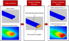 |
Fig. 1 Main steps of element deposition technique. |
2.1.2 Boundary condition and material properties
As material addition is modeled by element addition, it is possible to apply boundary conditions on every surface of the manufactured part (Fig. 2). This is an advantage over modeling methods such as inactive element method or quiet element method. Therefore, on every face of the meshed surface, convection and radiation are applied and updated after each deposition time step. The evolution of material properties such as conductivity, specific heat and density as a function of temperature is also taken into consideration.
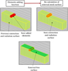 |
Fig. 2 External surface recalculation. |
2.1.3 Energy input
The energy used to melt wire and substrate is delivered through the creation of an electrical arc as it is common for electric welding processes. For this reason, the energy input model developed by Goldak for arc welding [22] has been adapted to the present model as commonly done for welding simulation [25–27]. Energy supply can be calculated by measuring the generator voltage, intensity and arc efficiency (U, I, ɳ). Moreover, according to Dupont [28], only 50% of the total arc power is delivered to the substrate via direct transfer, while the remaining 50% is used to melt the feed wire. Thus, the Goldak heat source is adapted and combined with the proposed element deposition technique to model the heat input taking into consideration the energy distribution between the wire and the substrate (Fig. 3).
Therefore, the direct energy transfer Qsource form the arc to the substrate is obtained considering the inferior half of the double-ellipsoid Goldak model. The remaining 50% of the total energy Qelements is delivered by means of the deposited elements modelling the droplet. An average deposition temperature modeling Qelements is calculated at each time-step. This deposition temperature considers the material properties previously presented. Qsource and Qelements are expressed in equation (1). (1)
(1)
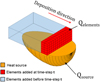 |
Fig. 3 Adapted Goldak heat source. |
2.1.4 Melt pool volume calculation
Based on the temperature maps provided by the finite element simulation after each deposition time-step, the volume of elements representing the melt pool (i.e., elements whose temperature exceeds the solidus temperature) is calculated, as illustrated in Figure 4. Thus, the evolution of the melt pool size can be monitored along the entire deposition process. As each calculated volume corresponds to a specific deposition time-step, linked to a specific position in the part total mesh. When additively manufacturing a thin wall, it is also possible to calculate the average volume value for each layer. This data named “mean melt pool volume” will be used as an indicator considering its correlation with the porosity rate for each layer.
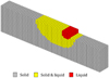 |
Fig. 4 Melt pool volume (yellow and red) = elements whose temperature exceeds the solidus temperature. |
2.2 Model validation
As the proposed model allows to record the whole thermal history of a production, a part is manufactured in order to validate the simulation. The part is designed as a thin wall of eight layers obtained by a zigzag strategy as illustrated in Figure 5. During the process, the temperature is measured in several points and compared to calculated values. Temperature measurements are done using six k-type thermocouples whose relative positions are shown in Figure 5.
5XXX aluminum alloys are used. An AA5083 grade has been chosen for the base plate composition. Thin wall part is built with a 1.2 mm wire in AA5356 aluminum alloy. Experiments are made using a WAAM cell composed by a Fronius CMT welding torch mounted on a Yaskawa MA1440 six-axis robot. Argon is used as inert gas with a flow of 25 L/min. The set of welding parameters are listed Table 1 and the arc efficiency was set to 0,83 [29]. These parameters are chosen to be close to the future use case of the simulation.
The AA5356 and AA5083 aluminum alloy used are assumed isotropic and temperature dependent. Nevertheless, in the absence of technical data in literature regarding the temperature dependent material properties of AA5356 alloy, and due to the similarities between the two alloys, the evolution of AA5083 conductivity, specific heat and density as functions of temperature is considered equal for both base and filler metals. Their values were obtained from El-Sayed work [30], and are presented in Table 2.
The considered aluminum alloys undergo a phase transformation over a range of temperatures, i.e. between solidus temperature (580 °C) and liquidus temperature (632 °C), with a latent heat of 380 kJ/kg. The phase transformation will be modeled by a latent heat of 380 kJ/kg and a constant temperature at 601 °C next referred as the melting temperature. Radiation to infinity is defined with an emissivity of ε = 0.77 and temperature of 20 °C. Convection is defined with a coefficient h = 20 Wm−2 K−1 and a temperature of 20 °C.
The evolution of the mesh and the corresponding temperature field can be visualized in Figure 6 at the first, second, seventh and the eighth layers.
Figure 7 gathers temperatures evolutions of the 6 measuring points, from P1 to P6, collected both by measurements and simulation.
A good agreement between experimental temperature and calculated is obtained. The average error is about 10%. The accuracy of the simulation can be considered sufficient for the evaluation of the thermal history of the part.
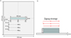 |
Fig. 5 Part geometry, trajectories and thermocouple positions to validate the finite element model: (a) Top view, (b) Front view. |
Welding parameters for model validation.
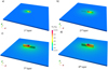 |
Fig. 6 Simulated temperature field of Zigzag strategy at different layers: (a) 1st layer, (b) 2nd layer, (c) 7th layer, (d) 8th layer. |
 |
Fig. 7 Measured and calculated temperatures at control points: (a) P1, P2 and P3 (b) P4, P5 and P6. |
3 Porosity vs melt pool volume evaluation
In order to analyze the correlation between the melt pool volume and porosity, experiments were conducted with different parameters influencing the thermal history of the fabrication. For each case, the mean melt pool volume is calculated at each layer using previous finite element model and compared with measured porosity of manufactured part. Two test cases are presented to study two different thermal condition.
3.1 Test cases
The two test cases are chosen in order to analyze two different porosity distributions. The test cases consist of manufacturing a 60-layers thin-walled part according to two different cooling time between layers (idle time). Welding parameters and trajectory strategy (zigzag) are identical for both cases, and idle times are changed from 2 s to 30 s. This must conduct to different thermal history in order to validate our hypothesis. The welding parameters are summarized in Table 3. The production means, the materials used, as well as the characteristic parameters are the same as those used in the validation experiment of the finite element model.
Test-case parts welding parameters.
3.2 Melt pool volume calculation and porosity measurement
The two test cases are simulated using the finite element model presented in this paper. The mean melt pool volume for each layer is calculated.
In the same time, the two parts are manufactured according their specific strategies. Then, a sample is extracted from each part using a saw (Fig. 8) in order to conduct a porosity analysis.
Each sample is analyzed thanks to X-ray tomography (RX Solutions Easytom XL). A microfocused source, whom tension and intensity have been kept constant at 150 kV and 66 μA, and a flat panel detector have been used. Acquisition conditions have led to a voxel size about 15 μm large. In order to visualized the whole sample height a helical scan has been performed implying 5760 projections over 8 rotations for the 30 s idle time sample (respectively 5000 projections and 5 rotations for the 2 s idle time sample). Each scan takes approximatively 45 min. A filtered-back projection algorithm has been used for reconstruction using the appropriate RX Solution software. Resulting illustrations of spatial distributions of pores are shown in Figure 9.
Furthermore, hydrogen content has been measured by inductively coupled plasma atomic emission spectroscopy (ICP-AES) in the mid-height and in the upper part of the sample (Tab. 4).
The simulated mean melt pool volume (MPV) and the measured porosity rate (in %) evolution along build direction for both strategies is plotted in Figure 10. As the final heights of the walls are not the same, the layer index is used to compared results. The layer index is recalculated considering that each layer has the same surface.
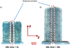 |
Fig. 8 Manufactured parts and sample definition: (a) idle time = 2 s, (b) idle time = 30 s. |
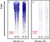 |
Fig. 9 Pores spatial distribution of both strategies (represented in blue): (a) idle time = 2 s, (b) idle time = 30 s. |
Hydrogen content measures.
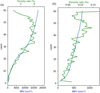 |
Fig. 10 Mean melt pool volume (MPV) and porosity rate evolutions according to layer number: (a) idle time = 2 s; (b) idle time = 30 s. |
3.3 Discussion
Results highlight a significant increase in the porosity rate along the build direction for parts produced with idle time 2 s rather than 30 s where the porosity is quite constant along the z axis. Observations reveal that pores become larger and numerous with the increasing number of layers in strategy 2 s, but they are much smaller and homogeneous, and their rate evolves very slowly along build direction in strategy 30 s [31]. The difference in the porosity defect evolution between the two strategies can be explained using the MPV evolution. As one can see from Figure 10, the MPV evolution can be correlated to the evolution of porosity rate. Indeed, in both strategies, the MPV and the porosity rate seem to evolve proportionally. They both increase as the part is getting taller, following the same dynamic. The Pearson coefficients are respectively 0.97 and 0.86 for idle time 2 s and 30 s on the 50th first layers. For the 2 s strategy, over the 50th layer, a gap can be observed between MPV and porosity rate. This can result of the limitation of the FEM model. Indeed, in the FEM model, bead width is assumed constant. This assumption is more fare from the reality over the 50th layer.
Moreover, microscopic observations reveal that the majority of detected pores are spherical, suggesting hydrogen trapping. The measures given in Table 4 and similar studies [32] highlight that, as shorter idle times induce heat accumulation and increased temperature and MPV in parts, hydrogen content evolves in the same way as porosity does. On the other hand, the introduction of longer idle-times (strategy 30 s) allowed to keep a small and quasi constant melt pool size, thus ensuring an equivalent amount of soluble hydrogen throughout the successive layers.
These correlations enable to validate the effectiveness of MPV variations as criterion for assessing the material integrity in terms of porosity of thin-walled aluminum parts produced by WAAM.
4 Conclusion
To conclude, this paper provides a simulation-based approach for the prediction of porosities during the production of aluminum parts by WAAM. After an analysis of the origin of porosity in aluminum WAAM manufacturing, a proposal is done that the monitoring of the porosity rate in aluminum WAMM effect can be achieved through melt pool volume monitoring. In order to calculate the MPV, thermal simulation of the WAAM process is proposed using finite element method. The proposed model is validated on an experimentation. In a second part, two test parts are chosen in order to access to two different pore distribution. These parts are manufactured and simulated. On manufactured part, a porosity measurement is done and MPV calculation is obtained from simulation result. For both cases, porosity rate regarding MVP is studied. Results show that, for a given manufacturing condition, the evolution of the melt pool volume and the evolution of the porosity are linked.
In conclusion, this paper shows that the melt pool volume variation is a good indicator to access to the porosity in wire arc additive manufacturing of aluminum part.
Results presented in this paper could be used in both academic research and industry. For example, to compare the risk of porosity for two given trajectories, or to help in the choice of welding parameters on a welding strategy. An integration of the MPV indicator in a simulation-based optimization algorithm can also be considered [33].
Future works may be to evaluate the influence of melt pool volume variation on shrinkage porosity. The present study focused on porosity due to hydrogen trapping but enlarge this approach to shrinkage pores could be a challenge. Indeed, this will need to use a very high tomography resolution or another measurement method.
In addition to the simulation of MPV variation as an indicator of porosity, work is underway to study in-process camera monitoring of the melt pool. This work should lead to a closed-loop system to control the porosity and the shape of the parts produced.
References
- B. Vayre, F. Vignat, F. Villeneuve, Designing for additive manufacturing, Proc. CIRP 3, 632–637 (2012) [CrossRef] [Google Scholar]
- T. Wohlers, I. Campbell, O. Diegel, R. Huff, J. Kowen, Wohlers Report 2021: 3D Printing and Additive Manufacturing Global State of the Industry, Wohlers Associates, Fort Collins, CO, USA (2021) [Google Scholar]
- S. Bau, D. Rousset, R. Payet, F.-X. Keller, Characterizing particle emissions from a direct energy deposition additive manufacturing process and associated occupational exposure to airborne particles, J. Occup. Environ. Hyg. 17, 59–72 (2020) [CrossRef] [PubMed] [Google Scholar]
- B. Wu, Z. Pan, D. Ding, D. Cuiuri, H. Li et al., A review of the wire arc additive manufacturing of metals: properties, defects and quality improvement, J. Manuf. Process. 35, 127–139 (2018) [CrossRef] [Google Scholar]
- K.E.K. Vimal, M. Naveen Srinivas, S. Rajak, Wire arc additive manufacturing of aluminium alloys: a review, Mater. Today Proc. 41, 1139–1145 (2021) [CrossRef] [Google Scholar]
- K. Derekar, J. Lawrence, G. Melton, A. Addison, X. Zhang et al., Influence of interpass temperature on Wire Arc Additive Manufacturing (WAAM) of aluminium alloy components, MATEC Web Conf. 269, 05001 (2019) [CrossRef] [EDP Sciences] [Google Scholar]
- M. Gierth, P. Henckell, Y. Ali, J. Scholl, J.P. Bergmann, Wire arc additive manufacturing (WAAM) of aluminum alloy AlMg5Mn with energy-reduced gas metal arc welding (GMAW), Materials 13, 2671 (2020) [CrossRef] [Google Scholar]
- Q. Wan, H. Zhao, C. Zou, Effect of micro-porosities on fatigue behavior in aluminum die castings by 3D X-ray tomography inspection, ISIJ Int. 54, 511–515 (2014) [CrossRef] [Google Scholar]
- R. Biswal, X. Zhang, A.K. Syed, M. Awd, J. Ding et al., Criticality of porosity defects on the fatigue performance of wire+arc additive manufactured titanium alloy, Int. J. Fatigue 122, 208–217 (2019) [CrossRef] [Google Scholar]
- X. Chen, F. Kong, Y. Fu, X. Zhao, R. Li et al., A review on wire-arc additive manufacturing: typical defects, detection approaches, and multisensor data fusion-based model, Int. J. Adv. Manuf. Technol. 117, 707–727 (2021) [CrossRef] [Google Scholar]
- K.S. Derekar, A review of wire arc additive manufacturing and advances in wire arc additive manufacturing of aluminium, Mater. Sci. Technol. 34, 895–916 (2018) [CrossRef] [Google Scholar]
- J. Bai, H.L. Ding, J.L. Gu, X.S. Wang, H. Qiu, Porosity evolution in additively manufactured aluminium alloy during high temperature exposure, IOP Conf. Ser. Mater. Sci. Eng. 167, 012045 (2017) [CrossRef] [Google Scholar]
- P.D. Lee, J.D. Hunt, Hydrogen porosity in directionally solidified aluminium-copper alloys: a mathematical model, Acta Mater. 49, 1383–1398 (2001) [CrossRef] [Google Scholar]
- L.-R. Hwang, C.-H. Gung, T.-S. Shih, A study on the qualities of GTA-welded squeeze-cast A356 alloy, J. Mater. Process. Technol. 116, 101–113 (2001) [CrossRef] [Google Scholar]
- Y. Zhao, Y. Jia, S. Chen, J. Shi, F. Li, Process planning strategy for wire-arc additive manufacturing: thermal behavior considerations, Addit. Manuf. 32, 100935 (2020) [Google Scholar]
- W. Hackenhaar, J.A.E. Mazzaferro, F. Montevecchi, G. Campatelli, An experimental-numerical study of active cooling in wire arc additive manufacturing, J. Manuf. Process. 52, 58–65 (2020) [CrossRef] [Google Scholar]
- X. Bai, H. Zhang, G. Wang, Improving prediction accuracy of thermal analysis for weld-based additive manufacturing by calibrating input parameters using IR imaging, Int. J. Adv. Manuf. Technol. 69, 1087–1095 (2013) [CrossRef] [Google Scholar]
- C. Xia, Z. Pan, J. Polden, H. Li, Y. Xu et al., A review on wire arc additive manufacturing: Monitoring, control and a framework of automated system, J. Manuf. Syst. 57, 31–45 (2020) [CrossRef] [Google Scholar]
- M. Graf, A. Hälsig, K. Höfer, B. Awiszus, P. Mayr, Thermo-mechanical modelling of wire-arc additive manufacturing (WAAM) of semi-finished products, Metals 8, 1009 (2018) [CrossRef] [Google Scholar]
- J. Xiong, Y. Lei, R. Li, Finite element analysis and experimental validation of thermal behavior for thin-walled parts in GMAW-based additive manufacturing with various substrate preheating temperatures, Appl. Therm. Eng. 126, 43–52 (2017) [CrossRef] [Google Scholar]
- F. Klocke, T. Beck, S. Hoppe, T. Krieg, N. Müller et al., Examples of FEM application in manufacturing technology, J. Mater. Process. Technol. 120, 450–457 (2002) [CrossRef] [Google Scholar]
- J. Goldak, A. Chakravarti, M. Bibby, A new finite element model for welding heat sources, Metall. Trans. B 15, 299–305 (1984) [CrossRef] [Google Scholar]
- A. Chergui, N. Beraud, F. Vignat, F. Villeneuve, Finite element modeling and validation of metal deposition in wire arc additive manufacturing, in Advances on Mechanics, Design Engineering and Manufacturing III, edited by L. Roucoules, M. Paredes, B. Eynard, P. Morer Camo, C. Rizzi (Springer International Publishing, 2021), pp. 61–66 [CrossRef] [Google Scholar]
- P. Michaleris, Modeling metal deposition in heat transfer analyses of additive manufacturing processes, Finite Elem. Anal. Des. 86, 51–60 (2014) [CrossRef] [Google Scholar]
- E. Cottier, P. Anglade, A. Brosse, E. Feulvarch, Fast 3D simulation of a single-pass steel girth weld, Mech. Ind. 17, 401 (2016) [CrossRef] [EDP Sciences] [Google Scholar]
- Y.G. Dehkordi, A.P. Anaraki, A.R. Shahani, Comparative study of the effective parameters on residual stress relaxation in welded aluminum plates under cyclic loading, Mech. Ind. 21, 505 (2020) [CrossRef] [EDP Sciences] [Google Scholar]
- D. Ding, S. Zhang, Q. Lu, Z. Pan, H. Li et al., The well-distributed volumetric heat source model for numerical simulation of wire arc additive manufacturing process, Mater. Today Commun. 27, 102430 (2021) [CrossRef] [Google Scholar]
- J. DuPont, A. Marder, others, Thermal efficiency of arc welding processes, Weld. J.-Weld. Res. Suppl. 74, 406s (1995) [Google Scholar]
- B. Mezrag, F. Deschaux Beaume, S. Rouquette, M. Benachour, Indirect approaches for estimating the efficiency of the cold metal transfer welding process, Sci. Technol. Weld. Join. 23, 508–519 (2018) [CrossRef] [Google Scholar]
- M.M. El-Sayed, A.Y. Shash, M. Abd-Rabou, Finite element modeling of aluminum alloy AA5083-O friction stir welding process, J. Mater. Process. Technol. 252, 13–24 (2018) [CrossRef] [Google Scholar]
- M. Limousin, G. Martin, P. Lhuissier, P. Robert, F. Vignat et al., Effect of wire arc additive manufacturing processing parameters on microstructure and porosity in a 5000 Al alloy, in 17th International Conference on Aluminum Alloys (2020) [Google Scholar]
- J. Gu, S. Yang, M. Gao, J. Bai, Y. Zhai et al., Micropore evolution in additively manufactured aluminum alloys under heat treatment and inter-layer rolling, Mater. Des. 186, 108288 (2020) [CrossRef] [Google Scholar]
- A.-T. Nguyen, S. Reiter, P. Rigo, A review on simulation-based optimization methods applied to building performance analysis, Appl. Energy 113, 1043–1058 (2014) [CrossRef] [Google Scholar]
Cite this article as: N. Béraud, A. Chergui, M. Limousin, F. Villeneuve, F. Vignat, An indicator of porosity through simulation of melt pool volume in aluminum wire arc additive manufacturing, Mechanics & Industry 23, 1 (2022)
All Tables
All Figures
|
Fig. 1 Main steps of element deposition technique. |
| In the text | |
|
Fig. 2 External surface recalculation. |
| In the text | |
|
Fig. 3 Adapted Goldak heat source. |
| In the text | |
|
Fig. 4 Melt pool volume (yellow and red) = elements whose temperature exceeds the solidus temperature. |
| In the text | |
|
Fig. 5 Part geometry, trajectories and thermocouple positions to validate the finite element model: (a) Top view, (b) Front view. |
| In the text | |
|
Fig. 6 Simulated temperature field of Zigzag strategy at different layers: (a) 1st layer, (b) 2nd layer, (c) 7th layer, (d) 8th layer. |
| In the text | |
|
Fig. 7 Measured and calculated temperatures at control points: (a) P1, P2 and P3 (b) P4, P5 and P6. |
| In the text | |
|
Fig. 8 Manufactured parts and sample definition: (a) idle time = 2 s, (b) idle time = 30 s. |
| In the text | |
|
Fig. 9 Pores spatial distribution of both strategies (represented in blue): (a) idle time = 2 s, (b) idle time = 30 s. |
| In the text | |
|
Fig. 10 Mean melt pool volume (MPV) and porosity rate evolutions according to layer number: (a) idle time = 2 s; (b) idle time = 30 s. |
| In the text | |
Current usage metrics show cumulative count of Article Views (full-text article views including HTML views, PDF and ePub downloads, according to the available data) and Abstracts Views on Vision4Press platform.
Data correspond to usage on the plateform after 2015. The current usage metrics is available 48-96 hours after online publication and is updated daily on week days.
Initial download of the metrics may take a while.