| Issue |
Mechanics & Industry
Volume 27, 2026
Artificial Intelligence in Mechanical Manufacturing: From Machine Learning to Generative Pre-trained Transformer
|
|
|---|---|---|
| Article Number | 11 | |
| Number of page(s) | 15 | |
| DOI | https://doi.org/10.1051/meca/2026005 | |
| Published online | 17 March 2026 | |
Original Article
Automatic modification and repair of three-dimensional models in intelligent manufacturing based on reinforcement learning
1
College of Media and Art Design, Guilin University of Aerospace Technology, Guilin 541004, Guangxi Zhuang Autonomous Region, PR China
2
School of Electronic Engineering and Automation, Guilin University of Electronic Technology, Guilin 541004, Guangxi Zhuang Autonomous Region, PR China
* e-mail: This email address is being protected from spambots. You need JavaScript enabled to view it.
Received:
16
August
2025
Accepted:
26
January
2026
Abstract
In intelligent manufacturing, the complex defects of three-dimensional models (such as holes, self-intersections, non-manifold edges/vertices, topological breaks, surface wrinkles, and normal anomalies) lead to low repair efficiency and poor manufacturing adaptability. This paper constructs an automatic repair method based on the PPO (proximal policy optimization) algorithm. Through the trust-domain constraint in PPO, the policy update divergence is avoided. Combined with a GNN (graph neural network), multi-scale geometric feature extraction, environmental perception, and dynamic decision-making are realized, thereby improving repair automation levels and manufacturing feasibility. The three-dimensional grid structure is topologically modeled using a GNN; local geometric features are extracted; and defect areas are identified. The reinforcement learning framework is applied to model the repair process as a state-action sequence decision problem, and the PPO algorithm is used to optimize the policy function and generate adaptive repair operations. The self-iteration mechanism is designed to realize multiple rounds of repair optimization and enhance the system’s robust processing capabilities for different types of defects. The experimental results show that when PPO+GNN is used to process typical complex defects such as holes, self-intersection overlaps, non-manifold edges and vertices, topological fractures, surface wrinkles, and normal anomalies, the boundary closure rate is between 0.7 and 0.9; the surface smoothness error is between 0.05 and 0.09; and there is high repair accuracy and geometric consistency. The printing success rate is between 0.85 and 0.95; the material utilization rate is between 0.77 and 0.82; and the manufacturing adaptability is good. The average number of convergence steps is 15; the total modification time is 5.8 s; the peak memory usage is 2.1 GB; and the repair efficiency and resource consumption are well balanced. The experimental data verify the effectiveness of the research presented in this paper on the automatic modification and repair of intelligent manufacturing 3D models.
Key words: Reinforcement learning / graph neural network / 3D model repair / intelligent manufacturing / proximal policy optimization / geometric consistency
© A.Z. Tan and B.S. Liu, Published by EDP Sciences, 2026
 This is an Open Access article distributed under the terms of the Creative Commons Attribution License (https://creativecommons.org/licenses/by/4.0), which permits unrestricted use, distribution, and reproduction in any medium, provided the original work is properly cited.
1 Introduction
The transformation, upgrading, and intelligentization of the manufacturing industry have led to higher requirements for the accuracy and repair efficiency of three-dimensional models. As the core foundation of intelligent manufacturing, the quality of three-dimensional digital models [1] directly affects subsequent processing, assembly, and product performance [2]. Complex structures and various defects have become bottlenecks that restrict the widespread application of three-dimensional models. Problems such as holes, non-manifold boundaries, and topological fractures frequently occur [3], leading to model discontinuities, surface roughness, and even unreasonable structures [4], which reduce manufacturing adaptability and product reliability. Faced with increasingly sophisticated design requirements, traditional rule-based and manual adjustment repair technologies have shown limitations, low repair efficiency [5], and a lack of universal processing capabilities for complex defects [6]. Therefore, automated and intelligent three-dimensional model repair technology [7] has become a key breakthrough in improving manufacturing efficiency and quality [8]. The development of technology has enabled graph neural networks (GNNs) to deeply mine local geometric information from topological structures [9], and the reinforcement learning framework can optimize policies in dynamic environments [10], providing new theoretical support and technical paths for the automatic repair of three-dimensional models. Combining the two, building an intelligent repair system that integrates environmental perception and dynamic decision-making can significantly improve the ability to handle complex defects, enable autonomous optimization of the repair process, and meet the needs of intelligent manufacturing for efficient, precise, and adaptable three-dimensional model repair [11].
Existing research has examined many aspects of automatic repair for three-dimensional models, focusing on defect detection, geometric completion, and topological repair [12]. Charton J proposed a MeshFix method that converted geometric problems into topological ones and performed local pairing operations on the topological graph, ultimately outputting a directional manifold mesh without inconsistencies. This method did not require the application of heuristic assumptions, retained the original geometric structure, and did not generate new inconsistencies or negative volumes [13]. Traditional geometric repair tools, such as MeshFix, are based on topological rules and geometric constraints and can repair simple holes and boundary defects [14], but their performance is limited when faced with complex topological structures and detail loss [15]. Sellán S applied a PSR (poisson surface reconstruction) method, which represented the reconstruction result as an improved Gaussian process, thereby supporting statistical reasoning and query of the reconstructed shape. This method not only improved the integration capability of traditional PSR in online scanning but also provided new ideas for integrating task priors and expanding applications [16]. The PSR method achieves smooth repair by reconstructing implicit surfaces, thereby improving the model’s smoothness, but its repair effect on large-scale [17], complex defects is limited [18]. Deep learning technology has gradually entered the field of three-dimensional models. Neural network models such as 3D-R2N2 [19] (3D recurrent reconstruction neural network) aim to learn repair policies from data to achieve end-to-end automatic repair and improve the ability to handle unstructured defects [20]. However, these methods have drawbacks, such as high computational overhead, limited generalization, and a lack of a dynamic environment-perception mechanism. They cannot fully meet the needs of intelligent repair of diverse defects in manufacturing scenarios, and there is still much room for improvement.
GNNs [21] are applied to extract local geometric features of three-dimensional models, as they can effectively handle non-Euclidean data and identify defective areas [22]. The reinforcement learning framework [23] provides theoretical support for dynamic decision-making in complex repair processes, enabling real-time adjustments to repair operations based on environmental feedback [24]. Existing studies have attempted to use deep reinforcement learning for model repair [25], mostly using policies based on DQN (Deep Q-Network) [26], A3C (asynchronous advantage actor-critic) [27], or DDPG (deep deterministic policy gradient) [28]. However, due to limitations in the discrete action space or unstable training, there is room for improvement in both repair effectiveness and efficiency. In addition, the mechanism of multiple rounds of repair iterations has not been fully explored, resulting in insufficient processing capabilities for complex defects. In prior work, the PPO algorithm has been widely used for optimization in continuous-action spaces due to its stability and efficiency [29]. Combining GNNs and reinforcement learning for graph structure optimization yields models with strong generalization and adaptability [30]. However, it remains challenging to directly apply these methods to the automatic repair of 3D models. The lack of a multi-round self-iterative repair mechanism limits the system’s comprehensive processing ability for complex defects and lacks a linkage evaluation system for geometric consistency and manufacturing adaptability during the repair process. This paper combines multi-scale geometric feature extraction from GNNs with a dynamic repair policy based on PPO [31], designs a self-iterative mechanism, and addresses the above shortcomings to build an intelligent 3D model automatic repair framework with high precision, high efficiency, and manufacturing adaptability [32].
This paper aims to develop a set of automatic 3D model modification and repair systems for intelligent manufacturing, overcoming the limitations of traditional repair technologies in complex defect processing and in manufacturing adaptability. By applying GNNs, fine-grained topological modeling of 3D grid structures is realized; multi-scale geometric features are precisely captured; and various defect areas are effectively identified. Combined with the PPO algorithm in reinforcement learning, the repair process is constructed as a state-action sequence decision problem; environmental perception and dynamic policy adjustment are realized; and the repair operation is ensured to be adaptive and robust. The innovative self-iterative repair mechanism enables the system to optimize repair results across multiple rounds, enhancing its comprehensive processing of complex, diverse defects. The system is systematically evaluated using indicators of repair accuracy, computational efficiency, and manufacturing adaptability, verifying the significant advantages of the method in improving the geometric consistency and manufacturing feasibility of three-dimensional models. Compared with traditional rule-based methods and deep learning models, this solution demonstrates stronger dynamic decision-making capabilities and greater practical application potential. Overall, the research not only offers an innovative technical approach to the automatic repair of three-dimensional models but also provides a solid theoretical foundation and practical solutions for the construction of high-quality digital models in intelligent manufacturing, thereby promoting the development of the manufacturing industry towards a more intelligent and refined direction.
2 Methods
Figure 1 systematically outlines the overall architecture for 3D model defect repair, covering topological encoding, environment modeling, policy generation, and self-iterative optimization. The original mesh data is transformed into a point-edge graph to extract key geometric features, and graph convolution is used to identify potential defect areas. The state vector is constructed based on the defect neighborhood topology, and indicators such as curvature change rate and boundary continuity are used as inputs to the policy network. The reinforcement learning algorithm is applied in the policy stage to evaluate state-action pairs, output refined local repair instructions, and set the reward function and feedback mechanism, in combination with geometric continuity and integrity. After each repair round, the system updates the defect score in real time, adjusts policy parameters, drives the next round of action generation, and performs dynamic adaptive repair of complex defect structures.
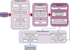 |
Fig. 1 3D model defect repair architecture. |
2.1 Topological encoding of 3D model defect area
The local topology of the defective area and its neighborhood is used as the environment-state input to the reinforcement learning agent, which constructs a state vector based on the local structure, including geometric indicators such as curvature change rate and boundary continuity, to enable the policy network to decide on the repair action.
2.1.1 Topological structure transformation and graph representation construction of three-dimensional mesh
A GNN is used to perform structured encoding on the original three-dimensional mesh data and construct a graph representation of vertices and edges. A three-layer graph convolutional network was adopted, with ablation experiments confirming its optimal configuration: fewer than three layers resulted in insufficient feature fusion, while exceeding three layers caused over-smoothing. Each layer expanded the neighborhood by one hop, resulting in a three-hop topology that ensured effective defect-detection coverage. More specifically, the 3D model’s mesh nodes are taken as the graph’s vertices, and the 3D model’s mesh boundary adjacency relation is used as edges to connect the vertices, which forms a point-edge graph. This guarantees topological closeness, that the adjacent information remains unchanged, and that the local features are preserved in subsequent processing. The hierarchical graph convolutional network sequentially processes graph-structured data layer by layer, exploiting information from neighboring nodes to summarize local geometric features, and it supports multi-dimensional attributes such as vertex normals, boundary closure, and curvature. The messages sent along edges in graph convolutional layers capture the local topological structure, which helps the network predict the exact locations of potential defect regions. The high-order representation of the node is obtained by averaging the geometric features of its neighboring nodes. The formula is defined as
 (1)
(1)
where  represents the feature representation of the node at the l-th layer; 𝒩(i) is the neighbor set of the node; cij is the normalization coefficient; W(l) is the weight matrix of the l-th layer; and σ is the activation function. This design can not only capture the complex dependencies between nodes but also enhance the model’s ability to identify local structural details, allowing defect features to be effectively extracted.
2.1.2 Geometric attribute extraction and defect area identification policy
The multi-scale geometric feature fusion technology is used to deeply mine the graph data after topological encoding to identify abnormal areas in the grid, including the quantitative calculation of geometric quantities such as vertex normal vector deviation, boundary closure, and local curvature anomaly, which are used as feature inputs of graph nodes. The normal vector deviation is used to reflect the local changes in surface smoothness, and the quantitative formula is defined as
 (2)
(2)
where ni is the normal vector of the node and is the set of its neighborhood nodes. This indicator shows an abnormal increase when sharp deformation or depression occurs on the node surface. Boundary closure evaluates the integrity of the node neighborhood boundary, reflecting whether there are openings or gaps, and local curvature anomalies capture the mutation points of the surface curvature. These geometric quantities are combined with the GNN’s output features, and a threshold-based judgment and anomaly detection mechanism are used to precisely locate potential defect areas. The specific steps are: use the joint expression of the node feature vector and the geometric index, design a defect scoring function, quantitatively score each node, and screen out areas with scores above the preset threshold as defect candidate areas. This method effectively avoids misjudgment from a single indicator and ensures the stability and accuracy of detection results through multi-scale feature fusion. In addition, the graph’s connectivity characteristics are used to cluster and group defect nodes, determine the spatial extent of the defects, and provide precise positioning support for the repair operation.
Table 1 lists in detail the key technical parameters involved in the topological encoding process of the defective area of the three-dimensional model, covering the structure construction and feature extraction links. The number of mesh vertices determines the complexity of the graph structure, which directly affects the sparsity of the point-edge graph and the geometric restoration ability of the model; the normal vector dimension is always kept in three dimensions to ensure the complete expression of spatial direction information; the node feature dimension is set at different stages according to the hierarchical structure of the graph neural network, supporting multi-level representation from local geometry to global structure; and the normalization coefficient range is used as a regulatory factor in the information aggregation stage to effectively alleviate the information imbalance caused by degree deviation. Preliminary experiments show that the range below 0.15 leads to insufficient information transmission, while above 0.95 may cause gradient saturation. The range of 0.15–0.95 effectively regulates the aggregation intensity of higher-order neighborhoods, balancing local detail preservation with global structural stability.
Parameters of topological coding technology for defect area detection.
2.2 Dynamic modeling of repair environment state
The local topology of the defective area and its neighborhood is used as the environment state input to the reinforcement learning agent model to construct a state vector based on the local structure, including geometric indicators such as curvature change rate and boundary continuity, for the policy network to decide on the repair action.
2.2.1 State vector construction of local topological structure
The local topological relationship of the defective area and its neighboring mesh nodes is extracted as the dynamic environment state input. A certain range is extended from the defect boundary, and the involved nodes and their connections are collected to form a local subgraph, ensuring the repair action can be performed in a complete, continuous mesh environment. For this subgraph, a multi-dimensional state vector is designed to fully reflect the structural changes and geometric characteristics. The core of the state vector includes indicators such as curvature change rate and boundary continuity, which measure the local deformation trend and boundary smoothness. The curvature change rate quantifies the rate of change of the geometric surface by comparing the time series of curvature at adjacent nodes. Its expression is
 (3)
(3)
where  represents the curvature value of the node at time t, and Δt is the time step, number of iterations. This indicator reveals the dynamic characteristics of deformation during the local surface repair process and helps the decision-making system grasp the trend of morphological evolution. Boundary continuity detects breaks or missing conditions by calculating the integrity of the connection between adjacent boundary nodes. The specific implementation is to count changes in the number of local boundary nodes and the degree of closure of boundary links as part of the state vector to measure changes in boundary continuity before and after repair. The vector of multi-dimensional state quantities is standardized and fed to the reinforcement learning agent to ensure a uniform scale for the input data, facilitating efficient training and accurate neural network predictions. This structured dynamic state representation directly reflects the immediate geometric changes in the repair environment and provides rich contextual information to support policy decision-making.
2.2.2 State response and action decision mechanism of policy network
The policy network [33] uses the constructed local state vector to dynamically adjust the repair action. After receiving input on the environment state, the network extracts implicit features via multiple layers of nonlinear transformations to develop a deep understanding of the local topological structure [34]. The action space comprises repair operations (including node adjustment, boundary stretching, and topological reconnection) that can accommodate a wide range of repair requirements for different types of mesh defects. The policy output, which is the priority of each action on the probability distribution, is updated gradually so as to maximize the long-term repair quality. The process of action selection integrates state information. Morphological adjustment actions are taken to smooth the surface for high-rate boundary curvature variation; boundary closure procedures are reinforced to close gaps for decreasing boundary continuity. This mechanism guarantees that the repairing action is well-tailored for the current state of the environment, as well as the precision and efficiency of the repair effect. After the action is performed, the environment state is updated in real time to generate closed-loop feedback, which leads the policy network to gradually learn and optimize repair paths across repeated iterations.
The policy network’s training objective is to maximize the cumulative repair benefit. The reward function in reinforcement learning is used to evaluate the effect of an action. The specific reward function uses the geometric error of the defect area and improvements in topological integrity as indicators. The form of the reward function is
 (4)
(4)
where Et is the geometric error indicator at time t, Ct is the topological integrity score, and α and β are the reward weights. This function guides the network to balance morphological accuracy and structural integrity during the repair process and promotes the policy to gradually converge to the optimal state. The fine design of the state vector and the synergy of the adaptive action decision of the policy network effectively improve the dynamic response capability and overall performance of defect repair.
Table 2 lists the training parameters and sampling configuration of the policy network. The state vector dimension is unified to 12, covering key geometric topological indicators. The action decision step frequency is strictly synchronized with the state sampling to ensure that the policy response is consistent with the environmental changes. The reward function adopts a dual structure, giving different weights to geometric error and topological continuity, respectively, adjusting the proportion to 0.7 and 0.3 to strengthen the guidance of structural integrity, Through grid search with 0.1 step size in the interval [0.5, 0.9], it is found that this ratio has the best comprehensive performance, which balances geometric accuracy and topological integrity and avoids excessive smoothing or structural distortion. In the training phase, the batch size is controlled to 64 to balance stability and efficiency. The learning rate is initialized to 0.001 and dynamically adjusted according to the policy feedback to ensure the network’s convergence performance and adaptability.
Policy network training parameters and sampling configuration.
2.3 Optimization of reinforcement learning policy and generation of repair actions
The policy function is optimized based on the PPO algorithm, and the action value is evaluated for each state. Local repair operation instructions are output, such as vertex translation, patch generation, and mesh merging. The reward function is applied in the reinforcement learning training process to measure the geometric continuity and integrity of the repaired model.
2.3.1 Dynamic update of policy function and action value evaluation
The update of the policy function is completed through an interactive sampling process. After the current state is input into the network, a set of action distribution probabilities is generated through the feature mapping module. In each round of policy evaluation, the network calculates the value estimate of the sampled actions and dynamically adjusts the weight of the policy function according to the repair effect brought by the actions. The action value is calculated based on the long-term expected return, combined with the continuity improvement of the model structure and the reduction of geometric error after the repair operation. The clip ratio function is used to control the amplitude of the policy update to prevent the policy from collapsing due to too fast a policy update. The function is defined as
 (5)
(5)
where rt(θ) represents the probability ratio of the new and old policies; At is the advantage function estimate; and ε controls the update range, set ε = 0.2 as the tolerance threshold for policy update magnitude. When the ratio of new to old policies exceeds the [1−ε, 1+ε] range, truncation is applied to prevent large-step updates from causing training oscillations, thereby enhancing the convergence stability of the PPO algorithm under complex geometric perturbations. This structure makes the policy adjustment more stable and avoids falling into overfitting or gradient explosion at local extreme points. In each round of iteration, the network records the feedback performance of all executable actions in the current state, takes the geometric improvement amplitude and topological coherence improvement as evaluation indicators, and finally forms the action value ranking result. High-value actions are preferentially retained for subsequent training to improve the action selection accuracy and the policy’s global adaptability. The continuous state-action records are sampled for multiple rounds to construct a training set. On this basis, the policy network gradually optimizes the response to complex defects and accurately allocates repair resources to key areas.
2.3.2 Local repair action generation and command control mechanism
The action generation module samples specific repair instructions based on the output probability of the current policy function. The types of repair actions include vertex fine-tuning, local reconstruction, patch fusion, and topological connection repair. After the action is sampled, it is not executed directly, but a dynamic screening is performed in combination with the current local geometric features to exclude solutions that are incompatible with the local structure to ensure the geometric rationality of the operation. Let us take vertex translation as an example: the system first computes the normal vector field of the target region and generates a movement vector that best preserves the shape of the vector field under the expected direction of curvature change, minimizing distortion and preserving the original structural features. The procedure enforces constraints from differential geometry to guarantee that the stability of the local mesh is not compromised by the operation.
A joint multi-objective reward function is constructed as the training feedback to evaluate the quality of each repair operation. It combines the two factors, the decrease in geometric error and the “closure” of structural improvement, into a single expression:
 (6)
(6)
where Cafter and Cbefore represent the front-to-back measurements of mesh coherence; Eafter and Ebefore represent the front-to-back geometric errors of the local curved surface; and λ1 and λ2 are weight factors. During training, the reward function guides the agent to prioritize actions that optimize both curvature and structural coherence, avoiding misjudgment caused by oversmoothing or local topological disturbances. After each round of training, the policy network parameters are adjusted according to the action feedback, gradually forming the ability to sensitively identify and directionally repair different types of defects. In the actual deployment stage, the policy function can quickly judge the input state in real-time, output repair instructions that conform to geometric logic, and complete local grid adjustment operations within the microsecond response range to achieve high-fidelity reconstruction and continuous repair of the model structure.
2.4 Self-iterative adjustment mechanism of repair results
After each round of action execution, the model state is re-evaluated, and the policy is adjusted according to the new defect score to form an adaptive iterative optimization process, realize dynamic processing of multiple types of defects, and improve the overall repair coverage.
Figure 2 shows the complete process of the self-iterative adjustment mechanism in the three-dimensional model repair process. After executing the repair action, the system updates the model topology in real-time and recalculates the defect score. Whether to adjust the policy based on the score change is determined. If the score improves, the policy parameters are optimized, and the current policy is kept. This mechanism forms a closed-loop control with the support of reinforcement learning agents and continuously iterates until the termination conditions are met, ensuring the integrity and adaptability of the repair effect, reflecting high dynamic response capabilities and multi-type defect processing coverage.
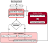 |
Fig. 2 Self-iterative adjustment mechanism. |
2.4.1 Real-time update of state reconstruction and defect scoring
After the local repair operation in each round is finished, the system reconstructs the current model state representation and re-extracts the structural information encoding local geometric consistency related to the fluctuation, boundary gradient perturbation, and curvature aggregation, along with the geometric center of gravity perturbation. The reconstruction of the state is not constrained to a region; the topological neighborhood of the region is included as well to detect precursors of degradation prior to being exposed to the domain perturbation. During this session, grain-scale modifications on patch aggregation patterns are applied as hints to bring new cracks or interface warping, originated by local repair, into the defect assessment sequence.
The defect scoring scheme uses a dynamic scoring vector to assign a distributed score to each area in which there could be a problem. In particular, the new scoring vector adds the state perturbation induced by the previous round of operation with the current geometric inconsistency to the repair response surface over the time interval, from which the local maximum rate of change is obtained, and the core region for the next round of operation is identified based on it. The specific scoring calculation is of the following form:
 (7)
(7)
where St(i) is the score of the previous round; ΔG(i) represents the geometric error increment of the current i-th area; and γ is the control factor. This update mechanism applies a sensitive response to real-time errors while maintaining the continuity of the scoring history, ensuring that the system can track new structural disturbances and make timely corrections. This structure avoids the omission of problems caused by traditional static evaluation of each region, extracts priority targets by comparing the fluctuation amplitude of the scoring, and enables the policy network to have clear repair direction guidance.
2.4.2 Multi-round adjustment path driven by policy feedback
After the scoring vector is updated, the system feeds back and adjusts the decision bias of the policy network according to the change trend. A weight modulation layer is applied in the policy execution module to dynamically reorder the original action distribution, increase the action probability of the region with significant score growth, and give priority to generating operation types that match its structural characteristics in subsequent sampling. This modulation does not rely on global retraining but rather updates the policy weights in a lightweight manner after each round of iteration to achieve a fast response to policy evolution.
To further improve the iteration effect, a global repair progress function Pt is applied to quantify the overall repair coverage and geometric coherence increment after each round of operation:
 (8)
(8)
where  and
and  represent indicators such as the front-back curvature discreteness or boundary fracture rate of the i-th region, and N is the number of valid regions. This function can quantify the contribution of this round of operations to the overall model state and serve as a reference for adjusting the policy step and action execution granularity. If a round of iteration produces a negative gain, the system reduces the action space and limits the operation range to avoid the impact of false repairs. If the positive gain is significant, the search radius is expanded, and the defect scoring threshold for the next round is increased to capture more extensive but hidden structural anomalies. The system implements a dual termination mechanism: it halts repairs when three consecutive rounds show improvement below 0.5% or when the preset maximum iteration count (default 20) is reached. This strategy balances repair completeness with computational efficiency, prevents infinite loops, and enhances algorithmic robustness.
3 Method effect evaluation
3.1 Experimental data and settings
The experiment uses multiple sets of 3D model datasets from the industrial manufacturing field, covering typical mechanical parts (such as gears, bearings, lock bodies, snow shovels, etc.). The model format is a triangular mesh with a vertex scale of 8000–45,000 to ensure the diversity and complexity of the data. The dataset contains six types of typical defects: holes, self-intersections, non-manifold edges/vertices, topological fractures, surface wrinkles, and normal anomalies. Each defect category (pores, self-overlapping, non-manifold edges/points, topological breaks, surface wrinkles, and normal anomalies) contains 20 samples, resulting in 120 model groups. This ensures equal representation of all defect types during training and testing, thereby enhancing evaluation fairness. The experimental environment is configured with an Intel Xeon E5-2680v4 processor, NVIDIA RTX 3090 (24 GB video memory), and 64 GB memory. The software platform is based on Python 3.8, PyTorch 1.12, and Open3D library.
The comparison methods select the traditional rule repair tool MeshFix, the implicit surface-based Poisson surface reconstruction (PSR), and the deep learning model 3D-R2N2. All methods are run on the same dataset, and the main evaluation indicators include boundary closure rate (the proportion of closed boundaries after repair), surface smoothness error (normal vector standard deviation), printing success rate (additive manufacturing simulation pass rate), and material utilization rate (repair volume/original volume).
3.2 Relationship between geometric anomaly pattern and feature coupling of three-dimensional mesh surface and feature changes of graph convolution nodes
The mesh of the three-dimensional industrial part model is reconstructed. The model surface is discretized into a standard triangular mesh structure, and the normal vector of each vertex is extracted. The local direction deviation is calculated in combination with its adjacent face normal vectors to construct the normal vector deviation matrix. At the same time, the curvature anomaly of each point is estimated by Gaussian curvature, and the degree of closure of the boundary ring is analyzed based on the topological adjacency relationship to obtain the boundary closure index. After all data are standardized, they are input into the graph neural network architecture for spatial feature encoding, and the results are used to draw three-dimensional deviation surfaces and multi-feature correlation distribution. This process takes into account both geometric information extraction and topological structure quantification to ensure that the data is comparable and engineering interpretable.
Figure 3 shows the coupling relationship between the geometric anomaly pattern and the features of the 3D mesh surface, and the colors represent the normal vector deviation.
Figure (a) intuitively shows the distribution of the normal vector deviation in the model surface space through the three-dimensional surface. The coordinate axes X and Y correspond to the spatial position of the discrete grid on the model surface, and the Z axis represents the normal vector deviation of the corresponding point. It is observed that the normal vector deviation in the central area is significantly higher than that in the periphery, indicating that the direction of the surface changes dramatically there, and there may be obvious geometric anomalies or defects. As the distance from the center increases, the deviation gradually decreases, indicating that the surface tends to be smooth and regular. The spatial distribution of this deviation is a reflection of the complex geometry of the model surface and provides crucial information for the location of potential defects. Figure (b) demonstrates the interdependence of three significant geometric features, i.e., normal vector deviation, curvature anomaly, and boundary closure. The aggregation of data points shows a certain nonlinear structure, which also suggests that these features are not separated in the modeling process but compound to represent the geometric wholeness and anomalous form of the model. A strong positive correlation trend is observed between the normal vector deviation and the curvature anomaly, indicating that locally curved surfaces generally experience drastic directional deviation. 0 boundary closure and normal vector deviation The boundary closure tends to be negatively correlated to the two other features, indicating that boundary irregularity and anomalous features in the other two measures can be found simultaneously. The transformation of the data effectively captures the subtle correlation of multi-dimensional features, and thus it also enables reasoning by graph neural networks to accurately encode and decode topological defectiveness. Additionally, Pearson correlation coefficient matrices were calculated separately for normal and defective regions. The results showed that normal deviation was strongly correlated with curvature anomalies (r = 0.83), while boundary closure exhibited a negative correlation (r = −0.71), confirming the statistically significant nonlinear clustering trend.
The normal vector deviation, boundary closure, and curvature anomaly are combined into the initial attribute vector of the node to form the original input data. The multi-layer graph convolution operation of the graph neural network is applied, and the adjacency matrix is used to describe the topological relationship between nodes. The node features are weighted, aggregated, and smoothed. The graph convolution kernel updates the node features through local neighborhood information so that the representation of each node integrates the features of the surrounding neighbors and reduces the noise caused by local anomalies. After iterating multi-layer graph convolution, the spatial distribution of node features tends to be smooth and continuous. The influence of abnormal points is effectively suppressed, and the structural characteristics of the defective area are highlighted.
Figure 4 shows the distribution of the original node features and the node features after graph convolution in two-dimensional space. The horizontal and vertical axes correspond to the spatial coordinates of the nodes in the two-dimensional plane, showing the actual distribution position of the nodes in the model. Figure (a) shows the spatial distribution of the initial node features. The feature values are reflected by color, with obvious local outliers and strong discreteness. The color distribution does not show obvious aggregation or diffusion trends, and the local high-value anomalies are clearly visible, indicating that the initial features have large fluctuations, and the correlation between adjacent nodes is not considered. The node feature basis displayed by the data reflects the differences in the original geometric properties of each node in the input three-dimensional model. Figure (b) shows the spatial distribution of node features after graph convolution. The color changes tend to be smooth; the feature values of abnormal nodes are effectively smoothed in the neighborhood; and the local extreme values are significantly weakened, forming a coherent gradient block. This process reflects the role of graph convolution in capturing topological structure information and fusing the features of neighboring nodes, effectively reducing the impact of noise and anomalies on feature recognition. The comparison of data reveals the contribution of graph convolution to topological coding. The smoothed features are more suitable for the identification of subsequent defect areas, which helps to accurately capture geometric anomalies and improve the robustness and accuracy of the model in defect detection.
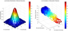 |
Fig. 3 Geometric anomaly pattern and feature coupling relationship of 3D mesh surface. |
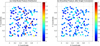 |
Fig. 4 Changes in the distribution state of node features after graph convolution. |
3.3 Dynamic evolution of geometric indicators, policy action probability, and repair effect
Multiple rounds of reinforcement learning repair experiments are conducted on the local topological structure of the defective three-dimensional model. For each repair time step, local geometric indicators, curvature change rate, and boundary continuity are collected, which are obtained by calculating the normal vector difference of adjacent vertices and the boundary closure function, respectively. These indicators reflect the dynamic changes of local surface smoothness and edge integrity and reflect the effectiveness of the repair process. The policy network action probability data comes from the output distribution of the policy network during the training process. For the three core repair actions (node fine-tuning, boundary stretching, and topology reconstruction), the probability values of the model selection at each time step are counted respectively, reflecting the emphasis and adjustment trend of the policy on different repair methods. By comparing the results of multiple rounds of iterations, the entire data reveals the mutual influence of environmental state changes and action distribution and verifies the dynamic adaptability and decision rationality of the model in complex three-dimensional defect repair, as shown in Figure 5.
Figure (a) shows the dynamic process of local curvature change and boundary continuity evolving over time in the repair task. The horizontal axis is the time step of the repair iteration; the left vertical axis is the curvature change rate; the right vertical axis is the boundary continuity index. There are large periodic oscillations in the curvature change rate at the beginning, reflecting that the policy network has strong instability when the local structure just starts to adjust; as the repair progresses, the change rate gradually decays and enters a stable fluctuation range, indicating that the surface tends to be smooth, and the structural disturbance is weakened. The boundary continuity decreases significantly in the initial stage, indicating that there are edge fractures or unclosed boundaries, but then it quickly recovers and tends to the original stable level, verifying that the boundary repair effect is gradually enhanced. The change in curvature and boundary continuity reflects the process in which the geometric environment state gradually changes from disorder to regularity under the action of the policy. Figure (b) depicts the evolution of the selection probability of the policy network for the three repair actions at different time steps. The probability of selecting the node fine-tuning action oscillates slightly, reflecting that the policy periodically optimizes the local grid points. The probability of the boundary stretching action is dominant in the early stage and is an important means to repair the open area. As the edge state improves, its role gradually decreases. The probability of the topological reconstruction action rises slowly from a low level and becomes the key to the policy decision in the later stage of repair, indicating that the model tends to repair the internal topological connection of the structure after the boundary is closed. The three together show the adaptive adjustment ability of the policy network: from edge completion to overall topological repair, the action distribution changes dynamically according to the environmental state, conforming to the logic of the gradually refined task process.
Figure 6 shows the repair effect of the 3D model automatic repair method in this study on two industrial parts. Figure (a) shows the repair process of the lock body model: the original model has obvious non-manifold boundaries, and the defective area is located by the topological features extracted by GNN. The PPO algorithm decides to perform node fine-tuning and boundary closure operations. The final repair result achieves dual optimization of surface continuity and topological integrity, and the lock structure restores the mechanical bite function of the design intention. Figure (b) is a snow shovel model repair case. After iterative repair, the policy network finally obtains a manufacturing-feasible model with a smooth surface and stable structure through topological reconstruction and curvature smoothing operations.
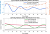 |
Fig. 5 Dynamic evolution of local geometric indicators and policy action probability during defect area repair. |
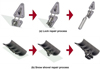 |
Fig. 6 3D model repair effect display. |
3.4 Evaluation of repair accuracy and geometric consistency
Repair experiments are conducted on multiple groups of 3D models containing different complex defects. For each type of defect, test samples of six typical problems, including holes, self-intersection overlaps, non-manifold edges and vertices, topological fractures, surface wrinkles, and normal anomalies, are collected. The repair capabilities of the PPO+GNN, MeshFix, Poisson surface reconstruction, and 3D-R2N2 methods in this paper are compared. Each method is run under the same dataset and unified evaluation criteria to ensure the comparability of the results. After the repair is completed, the proportion of unclosed boundaries after defect repair is quantified by calculating the boundary closure rate, and the surface smoothness error is measured by using the change in the standard deviation of the unit normal vector. The boundary closure rate is defined as the percentage of successfully closed boundary edges in the repaired model relative to the total number of boundary edges in the original defect region. During the experiment, a specially designed geometric analysis module is used to automatically extract boundary and normal information to precisely capture the detailed differences in the repair effect.
Figure 7 shows the comparative performance of two sets of key indicators on different complex defect types, namely boundary closure rate and surface smoothness error. Figure a reflects the ability of each repair method to recover boundary closure when dealing with multiple defects such as holes, self-intersections, non-manifold edges and vertices, topological fractures, surface wrinkles, and normal anomalies. The reinforcement learning method combining a graph neural network and policy optimization shows a higher boundary closure rate, with a value between 0.7 and 0.9, indicating that it can more effectively reduce the proportion of unclosed boundaries when repairing defects and ensure the model’s geometric integrity. In contrast, the closure performance of traditional methods under complex topological structures has certain fluctuations, which may be limited by the locality and singleness of its repair policy, and it is difficult to take into account the diverse characteristics of multiple defect types. Figure b shows the difference in surface smoothness error after repair by each method. The smoothness error reflects the stability and continuity of the normal vector change and is an important indicator for judging the quality of the details of the repair effect. Reinforcement learning with a graph neural network has more uniform results in error correction, with the values ranging from 0.05 to 0.09, which means its repairing action could positively reduce local geometric mutations and wrinkles and enhance the surface quality. The error rate for the other methods is high, and they perform highly fluctuating errors on the surface wrinkle defects, which indicates that the repairing process does not maintain continuity well. Repair methodology based on deep learning policy has great versatility and robustness against many types of complex defects, and it also enables the repaired model to possess enhanced overall structural integrity while meeting the geometric continuity, which is considered a more effective technical solution for high-precision three-dimensional model defect repairing.
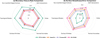 |
Fig. 7 Comparison of different complex defect types. |
3.5 Repair efficiency and computational complexity
The time required for each repair iteration and the overall computing resource consumption are counted, and the efficiency of the method is evaluated in combination with the algorithm convergence speed to ensure the practicality of intelligent repair. The performance of the four methods in this paper, PPO+GNN, MeshFix, Poisson Surface Reconstruction, and 3D-R2N2, in this regard, is compared.
The independent operation records of the four repair methods under the same defect dataset are recorded on a unified experimental platform. To ensure the fairness of the evaluation, representative multi-type 3D model defect instances are selected, and the complete repair process of each method is executed, respectively. An automated script is used to record the average iteration time, total repair time, peak memory usage, average convergence steps, and GPU (Graphics Processing Unit) usage in real-time. The convergence step determines the repair stop time by setting an error threshold. The computing resources are precisely collected by the system-level monitoring tool. All experiments are repeated three times, and the average value is taken as the final indicator. The platform hardware and software environment is fixed, including the same GPU model, memory configuration, and operating system, to ensure that the data results are stable and reproducible.
Table 3 quantitatively depicts the efficiency and computing resource consumption of different repair strategies, which are skewed from five aspects, namely the average iteration time, total repair time, peak memory usage, average number of convergence steps, and GPU usage. Results from all key indicators indicate that the proposed method is highly efficient for the overall processing. It converges orders of times faster with an average convergence step of 15, indicating a much stronger policy optimization ability. The time for a single repair to operate is short, so the overall time consumption is significantly reduced. The action generation mechanism is more precise, and the total repair time is 5.8 s. The memory usage control of the present invention is stable, with a peak memory usage of 2.1 GB and no drastic change, which illustrates that the present invention has a good space optimization policy in the state modeling and the graph structure processing. The GPU utilization, while high, stays within a reasonable range and does not overload, which confirms the method is able to better schedule resources for when it needs to perform both reasoning and action choosing in the more complicated topological world. On the other hand, the other three methods have longer convergence steps, and some methods need more total time consumption due to complicated reconstruction strategies or structural redundancy. The memory usage and computing load are relatively dispersed, which is not conducive to deployment and application in multiple scenarios. The data verify that the proposed method has good computational efficiency and system stability.
Quantitative comparison of efficiency and computing resource consumption.
3.6 Manufacturing adaptability index
PPO+GNN, MeshFix, Poisson surface reconstruction, and 3D-R2N2 are used to repair each type of defect model. Subsequently, the repaired model is input into the additive manufacturing simulation environment for printing feasibility evaluation, and the number of successful printings of the model under each type of defect is counted to calculate the printing success rate. The material utilization rate is defined as the ratio of the volume of the repaired model to that of the original intact (defect-free) model, which is used to measure the material retention efficiency during the repair process. All tests are completed under the same printing parameters and process simulation conditions to ensure the fairness of the evaluation and the comparability between methods.
Figure 8 shows the performance of the four repair methods in terms of manufacturing adaptability under multiple types of complex defects, which are evaluated from the two dimensions of printing success rate and material utilization. The columnar part reflects the ability of different methods to maintain geometric structure stability in additive manufacturing simulation. Among them, PPO+GNN shows higher consistency overall, with a printing success rate between 0.85 and 0.95. It has better geometric closurability and structural consistency in all complex defect problems, which greatly decreases the probability of failure in manufacturing. On the other hand, for multiple interference features (e.g., self-overlap and surface wrinkles), the conventional approach cannot finely model local topological information, leading to a drastic drop in printing stability. The dashed line part shows the differences in efficiency for different approaches in material utilization. PPO+GNN also enjoys better capability of material configuration for most defect states, with a material utilization ratio of about 0.77–0.82, and the reason is that the action policy of PPO+GNN dynamically avoids structural redundancy as well as local completion control, which leads to a repaired model with higher filling rationality. When faced with complicated boundaries and curvature discontinuities, these methods commonly lead to over-repair or under-repair and lower material usage or more support material facilitating material usage. The results indicate that PPO+GNN can not only enhance the stability of manufacturing after repair but also keep a relatively high efficiency in material utilization; hence, it has potential for applications in real manufacturing processes.
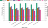 |
Fig. 8 Manufacturing adaptability performance. |
3.7 Dynamic decision-making ability quantification indicators
Using a unified model input process, four types of policy modules, PPO, DQN, A3C, and DDPG, are embedded, respectively. They are run under the same training round and hardware configuration, and the average policy update frequency, average response time, policy drift index (↓ meaning the lower is better), and action stability are recorded. The policy drift index is defined as the moving average of KL divergence (Kullback–Leibler divergence) between adjacent policy outputs, reflecting the volatility of the policy distribution. A lower value indicates more stable policy evolution, facilitating horizontal comparison of decision consistency across different algorithms. All experiments are completed in a GPU acceleration environment, and the sampling period is consistent with the state recording step size to ensure the timeliness and fairness of the comparison results. The final result takes the average of multiple rounds, and the extreme data is excluded to obtain a more representative performance.
The data in Table 4 compares the dynamic decision-making performance of different reinforcement learning policies. In terms of average policy update frequency and average response time, which are two important dimensions, the robust PPO approach achieves excellent stability and response speed, demonstrating its superior policy adaptive adjustment ability in relatively complex geometrical perturbation environments. This benefit can be attributed to its sheer update strategy that considerably reduces the policy oscillation and enhances the fault tolerance against the local state perturbation. Unlike DQN and DDPG, which demonstrate potential policy drift in topological mutation or local tampering, resulting in gradually unstable output actions, revealing that their convergence paths are more easily disturbed by the environment and hence fail to salvage planning consistently. Although A3C has some asynchronous updates and ranks higher in response delay compared to DQN, it still suffers from certain deficiencies in policy stability, as the action distribution experiences considerable fluctuations. To conclude, PPO is more appropriate for real-time response and policy update, demanding 3D defect repair tasks, and can be expected to be more reliable under more realistic scenes and different configurations.
Dynamic decision-making ability quantification.
4 Conclusions
This study focuses on the intelligent policy design in complex three-dimensional model defect repair, constructs an efficient repair framework driven by reinforcement learning policies, and combines it with graph neural network topology representation. This method significantly improves the sensitivity and discrimination of defect recognition by finely extracting local structural geometric features and establishing a state space expression mechanism. In the policy generation and action selection stages, the model is strengthened to have the ability to respond quickly to complex environments and maintains adaptability and robustness to multiple types of defect scenarios through continuous policy updates. A self-iterative feedback mechanism is applied in the repair process, which effectively compensates for the local deviations caused by single-step repair based on dynamic scoring and policy adjustment and promotes the gradual recovery of overall geometric continuity. When combining graph neural networks and PSO methods to process typical complex defects such as holes, self-intersections, non-manifold edges and vertices, topological fractures, surface wrinkles, and normal anomalies, the boundary closure rate is between 0.7 and 0.9; the surface smoothness error is between 0.05 and 0.09; the printing success rate is between 0.85 and 0.95; and the material utilization rate is between 0.77 and 0.82, verifying the good performance of this method in repair accuracy and manufacturing adaptability. The comparison results show that this method exhibits stronger generalization ability and policy stability when dealing with complex defect model structures. This method has established a relatively systematic technical path in intelligent repair decision-making, complex topological structure recognition, and geometric consistency optimization, providing technical support and a method framework with practical value for application scenarios such as three-dimensional model reconstruction and digital manufacturing pre-processing. Future work can focus on integrating multi-source heterogeneous data and self-supervised learning to further improve the intelligent repair system’s generalization ability and autonomous adaptation level.
Funding
This research was funded by Research foundation ability improvement project of Young and middle-aged teachers in Guangxi Colleges and Universities in 2022: “Research on virtual Display of Baibuyao Cultural Tourism Scenic Spot in Guangxi under the Rural Revitalization Strategy”, Project number: 2022KY0778.
Conflicts of interest
The authors have nothing to disclose.
Data availability statement
No data were used to support this study.
Author contribution statement
Conceptualization, Zhongxuan Tan, and Shilong Liu; Methodology and Software, Shilong Liu; Validation, Zhongxuan Tan; Formal Analysis, Shilong Liu; Investigation, Zhongxuan Tan; Resources, Shilong Liu; Data Curation, Shilong Liu; Writing – Original Draft Preparation, Shilong Liu; Writing – Review & Editing, Zhongxuan Tan; Visualization, Zhongxuan Tan; Supervision, Shilong Liu.
References
- Y.H. Son, G.Y. Kim, H.C. Kim et al., Past, present, and future research of digital twin for smart manufacturing, J. Comput. Des. Eng. 9, 1–23 (2022) [Google Scholar]
- S. Kumar, T. Gopi, N. Harikeerthana, M.K. Gupta et al., Machine learning techniques in additive manufacturing: a state of the art review on design, processes and production control, J. Intell. Manufac. 34, 21–55 (2023) [Google Scholar]
- L. Chen, Y. Zhao, X. Chen et al., Repair of spline shaft by laser-cladding coarse TiC reinforced Ni-based coating: process, microstructure and properties, Ceram. Int. 47, 30113–30128 (2021) [Google Scholar]
- A. van Oudheusden, J. Bolaños Arriola, J. Faludi et al., 3D printing for repair: an approach for enhancing repair, Sustainability 15, 5168–5201 (2023) [Google Scholar]
- S.F. Iftekar, A. Aabid, A. Amir et al., Advancements and limitations in 3D printing materials and technologies: a critical review, Polymers 15, 2519–2542 (2023) [Google Scholar]
- A. Kantaros, P. Zacharia, C. Drosos et al., Smart infrastructure and additive manufacturing: synergies, advantages, and limitations, Appl. Sci. 15, 3719–3754 (2025) [Google Scholar]
- M.H. Ali, G. Issayev, E. Shehab et al., A critical review of 3D printing and digital manufacturing in construction engineering, Rapid Prototyp. J. 28, 1312–1324 (2022) [Google Scholar]
- W. Qin, Q. Hu, Z. Zhuang et al., IPPE-PCR: a novel 6D pose estimation method based on point cloud repair for texture-less and occluded industrial parts, J. Intell. Manufac. 34, 2797–2807 (2023) [Google Scholar]
- H. Wang, Innovative application of intelligent mechanical manufacturing based on self-supervised learning and graph neural network fusion optimization, Informatica 49, 1–14 (2025) [Google Scholar]
- M.A. Masalha, K.K. VanKoevering, O.S. Latif et al., Simulation of cerebrospinal fluid leak repair using a 3-dimensional printed model, Am. J. Rhinol. Allergy 35, 802–808 (2021) [Google Scholar]
- M. Milazzo, F. Libonati, The synergistic role of additive manufacturing and artificial intelligence for the design of new advanced intelligent systems, Adv. Intell. Syst. 4, 1–7 (2022) [CrossRef] [Google Scholar]
- D. Mazzaccaro, F. Sturla, A. Rosato et al., Planning the use of endografts in the endovascular repair of complex abdominal and thoraco-abdominal aortic lesions leveraging 3D printing, Expert Rev. Med. Devices 21, 1121–1130 (2024) [Google Scholar]
- J. Charton, S. Baek, Y. Kim, Mesh repairing using topology graphs, J. Comput. Des. Eng. 8, 251–267 (2021) [Google Scholar]
- P. Wang, M. Xu, S. Xin et al., Robustly watertight manifold surface repair, J. Comput. Aided Des. Comput. Graph. 36, 1047–1056 (2024) [Google Scholar]
- X. Wang, N. Lei, Z. Luo, An automatic surface-based mesh repairing algorithm, J. Comput. Aided Des. Comput. Graph. 34, 1391–1401 (2022) [Google Scholar]
- S. Sellán, A. Jacobson, Stochastic Poisson surface reconstruction, ACM Trans. Graph. 41, 1–12 (2022) [Google Scholar]
- A. Farshian, M. Götz, G. Cavallaro et al., Deep-learning-based 3D surface reconstruction—a survey, Proc. IEEE 111, 1464–1501 (2023) [Google Scholar]
- H. Tian, C. Zhu, Y. Shi et al., Superudf: Self-supervised udf estimation for surface reconstruction, IEEE Trans. Vis. Comput. Graph. 30, 5965–5975 (2023) [Google Scholar]
- Q. Zou, F. Liu, 3D reconstruction of optical building images based on improved 3D-R2N2 algorithm, Teh. Vjesn. 30, 1594–1602 (2023) [Google Scholar]
- Y. Xi, H. Zhang, B. Li, Wear particles image enhancement using long short-term memory 3D recurrent reconstruction neural network (LSTM 3D-R2N2), Proc. Inst. Mech. Eng. C: J. Mech. Eng. Sci. 238, 10864–10872 (2024) [Google Scholar]
- C. Jian, Y. Lu, M. Lin et al., A novel graph neural networks approach for 3D product model retrieval, Int. J. Comput. Integr. Manuf. 36, 381–392 (2023) [Google Scholar]
- Y. Zhang, J. Chen, L. Chen et al., Automated structural repair based on continuous carbon fiber reinforced plastic 3D printing and online model reconstruction, Polym. Compos. 45, 13627–13638 (2024) [Google Scholar]
- L. Li, F. He, R. Fan et al., 3D reconstruction based on hierarchical reinforcement learning with transferability, Integr. Comput. Aided Eng. 30, 327–339 (2023) [Google Scholar]
- B. Felbrich, T. Schork, A. Menges, Autonomous robotic additive manufacturing through distributed model‐free deep reinforcement learning in computational design environments, Constr. Robotics 6, 15–37 (2022) [Google Scholar]
- A. Zhu, T. Dai, G. Xu et al., Deep reinforcement learning for real-time assembly planning in robot-based prefabricated construction, IEEE Trans. Autom. Sci. Eng. 20, 1515–1526 (2023) [Google Scholar]
- A. del Real Torres, D.S. Andreiana, A. Ojeda Roldan et al., A review of deep reinforcement learning approaches for smart manufacturing in industry 4.0 and 5.0 framework, Appl. Sci. 12, 12377–12407 (2022) [Google Scholar]
- S.R. Pokhrel, Learning from data streams for automation and orchestration of 6G industrial IoT: toward a semantic communication framework, Neural Comput. Appl. 34, 15197–15206 (2022) [Google Scholar]
- H. Shi, M. Yang, I. L. D. Makanda, W. Guo et al., Collective intelligence-driven 3D printing factory for social manufacturing: implementing a testbed for industrial application, Int. J. Comput. Integr. Manufac. 38, 362–385 (2025) [Google Scholar]
- W. Peng, W. Wang, Y. Wang et al., Key technologies and trends of active robotic 3-D measurement in intelligent manufacturing, IEEE/ASME Transac. Mechatronics 29, 4778–4799 (2024) [Google Scholar]
- X. Zhao, Z. Wang, The factory supply chain management optimization model based on digital twins and reinforcement learning, Scalable Comput. Pract. Exp. 26, 241–249 (2025) [Google Scholar]
- Y. Li, C. Yu, Flexible job shop scheduling with job precedence constraints: a deep reinforcement learning approach, J. Manufac. Mater. Process. 9, 216–241 (2025) [Google Scholar]
- Z. Guo, Y. Zhang, S. Liu et al., Exploring self-organization and self-adaption for smart manufacturing complex networks, Front. Eng. Manag. 10(2), 206–222 (2023) [Google Scholar]
- C.N. Idika, U.U. James, O.M. Ijiga et al., A. digital twin-enabled vulnerability assessment with zero trust policy enforcement in smart manufacturing cyber-physical system, Int. J. Sci. Res. Comput. Sci. Eng. Inf. Technol. 9, 1–25 (2023) [Google Scholar]
Cite this article as: A. Zhongxuan, B. Shilong Liu, Automatic modification and repair of three-dimensional models in intelligent manufacturing based on reinforcement learning, Mechanics & Industry 27, 11 (2026), https://doi.org/10.1051/meca/2026005
All Tables
All Figures
|
Fig. 1 3D model defect repair architecture. |
| In the text | |
|
Fig. 2 Self-iterative adjustment mechanism. |
| In the text | |
|
Fig. 3 Geometric anomaly pattern and feature coupling relationship of 3D mesh surface. |
| In the text | |
|
Fig. 4 Changes in the distribution state of node features after graph convolution. |
| In the text | |
|
Fig. 5 Dynamic evolution of local geometric indicators and policy action probability during defect area repair. |
| In the text | |
|
Fig. 6 3D model repair effect display. |
| In the text | |
|
Fig. 7 Comparison of different complex defect types. |
| In the text | |
|
Fig. 8 Manufacturing adaptability performance. |
| In the text | |
Current usage metrics show cumulative count of Article Views (full-text article views including HTML views, PDF and ePub downloads, according to the available data) and Abstracts Views on Vision4Press platform.
Data correspond to usage on the plateform after 2015. The current usage metrics is available 48-96 hours after online publication and is updated daily on week days.
Initial download of the metrics may take a while.