| Issue |
Mechanics & Industry
Volume 18, Number 5, 2017
|
|
|---|---|---|
| Article Number | 505 | |
| Number of page(s) | 13 | |
| DOI | https://doi.org/10.1051/meca/2017018 | |
| Published online | 04 September 2017 | |
Regular Article
Three-dimensional study of parallel shear flow around an obstacle in water channel and air tunnel
1
Research Unit of Metrology and Energy Systems, ENIM, University of Monastir,
5019 Kairouan Street,
Monastir, Tunisia
2
Research Unit of Ionized Backgrounds and Reagents Studies, University of Monastir,
5019 Kairouan Street,
Monastir, Tunisia
3
Thermal Centre of Lyon, National Institute of Applied Science of Lyon,
69621
Villeurbanne Cedex, France
* e-mail: This email address is being protected from spambots. You need JavaScript enabled to view it.
Received:
19
May
2016
Accepted:
27
March
2017
Abstract
The purpose of this study is to show the effect of some physical parameters on a parallel shear flow. The variation of the velocity inlet and the influence of an obstacle placed at the bottom of a channel were analyzed. The governing equations based on K–ε model in a line source downstream around a three-dimensional obstacle are determined by the finite volume method with SIMPLEC algorithm. The obtained results have allowed to establish the dynamic characteristics of this kind of flow. Horizontal and vertical velocity fields, Reynolds shear stress field, turbulence intensity and scalar concentration in the water channel and a wind tunnel were exposed. These results permit us to localize the maximum and minimum zones of turbulence, which help us to exploit those fields for different purposes such as energy extraction and port infrastructure.
Key words: shear flow / turbulence / finite-volume method / K–ε model / Reynolds shear stress / scalar concentration
© AFM, EDP Sciences 2017
1 Introduction
Shear flow is developed in most of the flows that govern our environment such as rivers, oceans or atmosphere. It also reveals a large number of industrial flows (aeronautical, energy, water) as an important parameter. The shear flows are heterogeneous flow with average velocity gradients, such as the jet of an erupted volcano and the exhaust gases of reaction engines in motion. Environmental and hydrodynamic assessment of the coastal fringe area degraded by rivers estuaries, pollution dispersion [1] as well as the wide use of obstacles in industrial and energy applications lead us to study the hydrodynamic phenomena that are formed when a shear flow encounters a fixed obstacle at the bottom of the water channel or a wind tunnel. In fact, many studies have been conducted to develop numerical models of shear flows [2]. There are generally three classes of models: first phase resolution models [3] or hydrodynamical models are based on extended Boussinesq equations that show the instantaneous movements of the fluid whatever the depth. Second the averaged phase models [4] or morphodynamical models are usually used in oceanic and continental seas similar to stochastic models [5] which are used to solve the energy propagation equation and allow considering the generation phenomena, dissipation and energy transfer present in deep water. Third the coupled morpho-hydrodynamical model [6] was applied for two models (shallow water equations and the extended Boussinesq equations) and used to simulate the movement of physical sandbars observed at Rousty beach (Mediterranean French coast). Nowadays, these models are common in coastal area by taking into account the terms associated with shallow water propagation (bathymetric wave breaking [7]). For the water flow (Fig. 1a), the experimental measurements of [8] were based on LIF (laser-induced fluorescence) [9]; for the air tunnel (Fig. 1b), the physical principle on which it is based the measurement of scalar flow is MSD (Mie scattering diffusion) [10]. As far as we know, the study of shear flows in the presence of obstacle was not sufficiently detailed numerically. The aim of this work is to explain, through a numerical simulation, the dynamic profile of a shear flow around a cubic obstacle installed at the bottom of a water channel or an air tunnel. Essentially, we want to show the capabilities of gradient transport modeling [11] in predicting atmospheric dispersion in complex flow and the influence of inlet velocities on the perturbation of the shear flow. Practically we are trying to show numerically the change on the profile of the horizontal and vertical velocity, as well as the Reynolds stress field, turbulence intensity and scalar concentration, which allow us to predict atmospheric dispersion in a shear flow. The first part of this report is devoted to a presentation of the physical model and different equations that control the shear flow. The second part deals with the validation of numerical model for a fixed inlet velocity with the experimental results of Vinçont et al. and the numerical results of Rossi and Iaccarino. The third part focuses on the obtained results and the interpretations for the different inlet velocities.
 |
Fig. 1 Physical model of: (a) water channel and (b) air tunnel. |
2 Analyses
This section aims to briefly explain the phenomenology and theoretical approaches of a shear flow, the various physical models and the different mathematical and numerical techniques adopted to simulate this kind of flow. We place ourselves in the context of incompressible flows for which the velocity field has a zero divergence, although it is impossible to characterize the shear flow with a strictly analytical point of view, we could identify its principal properties of turbulent regime. Therefore the incompressible viscous flows of two continuous fluids, for example, air and water, are governed by mass conservation (continuity equation) and momentum conservation (Navier–Stokes equation) formulating classical conservation laws. To model the development of shear flows with variable density around an obstacle at the bottom of a channel, the finite volume method is adopted. However we must previously show the physical presentations of the problem surrounded by the boundary conditions for all the cases.
2.1 Physical presentation problem
The physical presentation of the proposed problem is shown in Figure 1. It describes two cuboids with a length L = 256 cm, width l = 306 mm for the water channel and 500 mm for the air tunnel, height H = 170 mm for water and 500 mm for the air, and a square section of barrier installed at the bottom of a channel at h = 7 mm for water and 10 mm for the air. The distance between the channel inlet and the first surface of the barrier is 130 h, the distance between the last surface of the barrier and the channel output is 234.7 h. The geometrical dimensions are those used by [8,11] for a Reynolds number Reh ≡ ∼ Ueh/ϑ = 700 for water channel and 1500 for the air tunnel, where Ue is the free stream velocity of the flow above the boundary layer and ϑ is the kinematic viscosity  for water and 1.46 × 10⁻⁵ m2 s−1 for the air. The thickness of the boundary layer, without the obstacle positioned at the bottom of channel is about 5 cm, so that δ/h = 7. This factor is the parameter that shows the length of the recirculation zone after the barrier where there is a large area of separation with the flow directed toward the opposite wall.
2.2 Mathematical model
It is assumed that the fluid is a continuous medium, viscous and Newtonian. Thus the dynamic viscosity is independent of strain rate and depends exclusively on the temperature and pressure; the three-dimensional and stationary flow around an obstacle is defined by the following equations:
Continuity equation:
 (1)
(1)
Momentum equation:
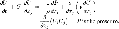 (2)
with i = 1, 2, 3.
(2)
with i = 1, 2, 3.
To solve this system we proceed the Reynolds rules, which state that, any instantaneous component of the flow (velocity, pressure, etc.) is a sum of two components: the first is an average and the second is a fluctuation.
 (3)
(3)
We can simplify and apply the Reynolds rules to obtain the following averaged equations of continuity and momentum:
Averaged continuity equation:
 (4)
(4)
Averaged momentum equation:
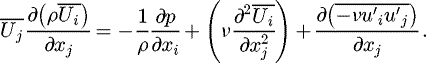 (5)
(5)
The determination of the equation is more complicated on account of the creation of additional unknown called Reynolds stress  , hence the need for a turbulence model to solve the system equation. The well identified SIMPLEC algorithm is used for pressure–velocity combination. The successive numerical equation systems are solved iteratively in a chronological approach. The results are obtainable for a flow in a channel with a moving indentation; they explain favorable harmony with experimental interpretation. The finite-volume method [12] can be exploited for both the Lagrangian and the Eulerian solution of the Navier–Stokes equation. The technique uses the integral shape of the governing equations for an arbitrary moving control volume, with pressure and Cartesian velocity components as reliant variables. Care is also taken to assure the space conservation rule, which ensures an entirely conservative numerical procedure. Completely implicit sequential differencing makes the technique steady for every time step. A full description is provided for the discretization in three dimensions, with a collocated collection of parameters. Fundamental differences are used to calculate the dispersion and diffusion fluxes. After that we show the results of numerical simulations obtained through a calculation code performed on the fluid mechanics software ANSYS Fluent.
2.2.1 K–ε turbulence model
For our system, we have designated the K–ε standard model; it is a semi-empirical model that adopts the Boussinesq concept [13] combining the Reynolds stresses with a mean deformation rate:
 (6)
where
(6)
where  is the strain tensor and
  is the turbulent kinetic energy [14].
The turbulent viscosity, defined by a velocity  and a distance
  , is given by:
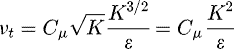 with Cμ = 0.09 and ε is the dissipation rate.
Transport equation of the turbulent kinetic energy K:
 (7)
(7)
Transport equation of the dissipation rate ε:
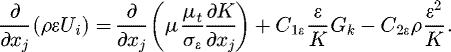 (8)
(8)
σk = 1, σϵ = 1.3 are, respectively, the numbers of Prandtl [15] related on the turbulent kinetic energy and the dissipation rate.
C1ϵ = 1.44, C2ϵ = 1.92 are empirically calculated values.
Gk is the production term given by
 (9)
(9)
Wind and water engineers usually exploit the K–ε model to numerically modelize the atmospheric boundary layer. Commercial softwares are perfectly exploited with wall functions used to model the surface of the irregular ground. Unlike earlier turbulence models, K–ε model focuses on the mechanisms that involve the turbulent kinetic energy. The principal assumption of this model is that the turbulent thickness is isotropic, in other words, the ratio between Reynolds stress and mean rate of deformations is equal in all directions. In order to discretize the equations of antecedent mathematical model, the finite volume method [16] is used for the mass conservation equations and the momentum equations, in all finite volume throughout the calculation domain. These equations are solved by the Gauss–Seidel method [17] by adapting an implicit scheme in time and space.
2.2.2 Choice and sensitivity of mesh
To ensure good results while keeping a reasonable calculation time, a non-uniform mesh was chosen. The grid is very tight around the obstacle where the gradient of the different variables is strong enough while it is rude elsewhere. For the resolution, the hybrid mesh generated by a mixture of elements of type tetrahedral, prismatic or pyramid in 3D, was selected (Fig. 2). This mesh combines the advantages of structured mesh with those of unstructured mesh. Indeed, this type of mesh is recommended to minimize the numerical errors in complex geometries [18]. Several simulations were performed for different numbers of meshes:
-
204 406, 336 793 and 387 846 nodes for the water channel;
-
404 219, 510 414 and 590 120 nodes for the air tunnel.
In Figure 3, there is plotted the variation of the horizontal velocity field in the water channel (Fig. 3a) and the air tunnel (Fig. 3b). The simulations were compared with experimental work [8]. A mesh of 336 793 and 510 414 nodes has been selected, respectively, for the water channel and the air tunnel, indeed with these mesh numbers the error with respect to [8] does not exceed 1%.
As shown in Figure 1 we used the inlet velocity used as a boundary condition at the inlet of the water channel and the air tunnel; at the output surface we take the output pressure for the water and air; at inferior limits and on the sides, is applied the wall boundary condition for water and air; at the upper limit we adopt the output pressure for the water channel and the wall boundary condition for the air tunnel. The Simplec algorithm [19] is admitted for the coupling of velocity–pressure. The second order upwind scheme [20] is chosen for convective and viscous expressions of each governing equation. It provides good solutions despite its difficulty to reach convergence. The complications of steady flows are generally determined by a pseudo temporal process or similar iterative representation given that the equations are nonlinear. An iterative representation is adopted to solve them. These techniques led to a successive linearization of the equations and the produced linear methods are often determined by iterative methods.
 |
Fig. 2 (a) Hybrid mesh in 3D and (b) zoom on the obstacle. |
 |
Fig. 3 Mesh sensibility on the horizontal mean velocity field after the obstacle for x = 4 h at the bottom of (a) a water channel and (b) an air tunnel. |
2.2.3 Analysis near the wall
The shear flows are very influenced by the presence of walls [21]. In close vicinity of the wall, fluctuations of tangential velocities are reduced by the fluid viscosity which incite a kinematic blocking that reduce perpendicular velocity fluctuations to the wall. But, away from the wall, turbulence intensifies abruptly by the multiplication of the turbulent kinetic energy due to gradients of high average velocity. For K–ε model, the equation of the turbulent kinetic energy K is determined for the entire domain with a condition on the wall given by  , where n is the normal local ordinate at the wall.
The production of the turbulent kinetic energy K and its dissipation rate ε (which recall the source terms in the equation of K) at the walls cells are calculated by using the condition of local equilibrium which requires the equivalence between the production of K and its dissipation rate in the cells.
Figure 4 verifies that the boundary layer on a wall [8,22,23] may be divided into three regions:
-
In close vicinity of the wall, for y+ < 15: U+ = y+ = Uτy/ν, where
 is the friction velocity.
In our case, the bottom of water channel and wind tunnel is flat and  [24] so the local skin friction τs is equal to the total wall shear stress τb, with η the height of bedform. A laminar under layer where the flow is completely laminar and fluid viscosity plays a major role in the transport of momentum, heat and mass.
-
Away from the wall, turbulence is predominant; the formula is valid for y+ > 250: U+ = 2.45, y+ + 5.54.
-
Between the two zones, there exists a region where turbulence and fluid viscosity have the same impact, for 15 < y+ < 250: U+ = lny+.
The curves in Figure 5 are obtained in the case where the fluctuations of tangential and normal velocities to the wall are correlated. The obtained results using K–ε model, in Figure 5, are fairly close for the entire domain to those of [8] that seem sensitive to the presence of high shear in the tests of the PIV image and which are considerably below the values of the direct numerical simulation (DNS) [25].
For the resolution, to avert the problem of the existence of wall, we are not going to solve the transport equations close to the wall (much-attenuated region by the viscosity) and we proceed to solve the transport equations with widely dense mesh throughout the walls; that is to say, we refine the mesh to the wall limits.
 |
Fig. 4 Profile of mean velocity field without obstacle: (a) in the water channel and (b) in the air tunnel. |
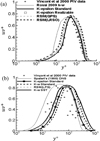 |
Fig. 5 Profile of Reynolds shear stress without obstacle: (a) in the water channel and (b) in the air tunnel. |
3 Results and discussion
The results of numerical simulations were obtained through a calculation code performed on the fluid mechanics software ANSYS Fluent. Our goal is to study the dynamic behavior of a shear flow around an obstacle placed at the bottom of a water channel and an air tunnel. Mainly, we are interested in the influence of the presence of the obstacle as well as the change of velocity inlet on the disturbance in the flow. For this, four cases were studied with different velocity values which are given as follows:
-
Case 1: Ue = Ue1 = Ue2 = 0.1 m s−1 for the water channel and Ue = Ue1 = Ue2 = 2.3 m s−1 for the air tunnel.
-
Case 2: Ue = Ue1 = 0.1 m s−1, Ue2 = 0 m s−1 for the water channel and Ue = Ue1 = 2.3 m s−1, Ue2 = 0 m s−1 for the air tunnel.
-
Case 3: Ue = Ue1 = 0.1 m s−1, Ue2 = 2Ue1 = 0.2 m s−1 for the water channel and Ue = Ue1 = 2.3 m s−1, Ue2 = 2Ue1 = 4.6 m s−1 for the air tunnel.
-
Case 4: Ue = Ue1 = 0.1 m s−1, Ue2 = ½Ue1 = 0.05 m s−1 for the water channel and Ue = Ue1 = 2.3 m s−1, Ue2 = ½Ue1 = 1.15 m s−1 for the air tunnel.
Our objective was to follow the influence of these velocities inlet on changing of these settings: Horizontal and vertical velocity fields, the shear Reynolds stress field, the turbulence intensity and the scalar concentration in a water channel and an air tunnel.
3.1 Flow field for Ue = Ue1 = Ue2
3.1.1 Contour of horizontal velocity field
Figure 6a–d, b–e and c–f show, respectively, the contours of the horizontal average velocity field for RSM, K–ω and K–ε turbulence models. It is observed that the velocity remains constant as from the entry of the canal until the first edge of the obstacle where there's a drop of the velocity due to the slowdown in the flow. So, a recirculation zone is formed after the obstacle at the bottom of the water channel and the air tunnel for the three turbulence models.
High velocity fields are detected above the obstacle to the upper limit of the domain. This velocity increase is explained by the narrowing of the passage surface due to the presence of the obstacle. It is noted that this high velocities area is limited in the K–ε model. In addition, the separation point of velocity for the three turbulence models is marked on the first edge of the obstacle. In return, the minimum values of the speed are situated after the obstacle forming the wake zone. We note that this recirculation zone decreases with the K–ε turbulence model.
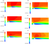 |
Fig. 6 Contour of horizontal velocity field around the obstacle in the water channel (a–c), in the air tunnel (d–f) for models (a, d) RSM, (b, e) K–ω, and (c, f) K–ε. |
3.1.2 Vertical component of average velocity field
Figure 7 shows the vertical average velocity fields for the different turbulence models for the abscissae x = 4 and 6 h located after the obstacle at the bottom of the water channel and the air tunnel. The obtained results using the K–ε model are the closest to experimental measurements of [8,22]. The four curves are almost superimposed throughout the height of the channel, which means that the vertical velocity is not disturbed by the obstacle. In this figure, we can differentiate two zones: in the lower half of the channel, a negative velocity was noticed and which explains the recirculation flow. On the contrary, the velocity increases in the upper part of the channel which is not disturbed by the presence of the obstacle. Hence we identify of the ordinate of separation at y = 0.01 m which is equal to the height of the obstacle at the bottom of the air tunnel and is greater than the height of the obstacle at the bottom of water channel.
 |
Fig. 7 Profile of vertical average velocity field after the obstacle at the bottom of: (a) a water channel for x = 4 h, (b) for x = 6 h, (c) an air tunnel for x = 4 h, and (d) for x = 6 h. |
3.1.3 Turbulence intensity field components
Figures 8 and 9 show the profiles of the horizontal and vertical turbulence intensity [26] for the various models of turbulence for the water channel and the air tunnel. According to the curves, it is observed that the turbulence intensity increases from the bottom wall of the channel to the upper limit of the obstacle. The turbulence increases slightly along the obstacle and then decreases for y > h. In general, we mark that the turbulence intensity is maximal in the interval between y/h = 1 and y/h = 1.5, but it is almost zero on the walls of the water channel and tunnel of air.
 |
Fig. 8 Profile of the turbulence intensity: (a) horizontal for x = 4 h, (b) x = 6 h, (c) vertical for x = 4 h, (d) x = 6 h; after the obstacle at the bottom of a water channel. |
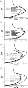 |
Fig. 9 Profile of the turbulence intensity: (a) horizontal for x = 4 h, (b) x = 6 h, (c) vertical for x = 4 h, (d) x = 6 h; after the obstacle at the bottom of an air tunnel. |
3.1.4 Reynolds shear stress
Figure 10 shows the profiles of the Reynolds shear stress [27] for various turbulence models for the abscissa x = 4 and 6 h. The obtained results using the K–ε model are in accord with experimental [8] and numerical measurements of [11]. The negativity of the Reynolds shear stress throughout the water channel and the air tunnel, indicates recirculation zone. And this results from the negativity of one of the two fields of vertical and horizontal velocity. The values of the Reynolds shear stress for the air tunnel are superior in terms of absolute values than that of the water channel given the difference of Reynolds number Reh.
 |
Fig. 10 Profile of Reynolds shear stress after the obstacle at the bottom of: (a) a water channel for x = 4 h, (b) x = 6 h, (c) an air tunnel for x = 4 h, (d) x = 6 h. |
3.1.5 Scalar dispersion
Figure 11 shows the profiles of the mean scalar concentration [28] for various turbulence models for the abscissa x = 4 and 6 h. The mean scalar concentration is increasing after the obstacle with values for x = 4 h higher than those for x = 6 h. It is elevated in the interval y/h = [0, 1.5], that is to say along the height of the obstacle and the length of recirculation zone which is maximal for y = h. Then this concentration decreases on the part above the obstacle until it vanishes at y/h = 3 for the K–ε model. The highest values of the scalar concentration for the air tunnel are lower than those of water channel considering the difference in the kinematic viscosity ϑ and the Reynolds number Reh.
 |
Fig. 11 Profile of the mean scalar concentration after the obstacle at the bottom of: (a) a water channel for x = 4 h, (b) x = 6 h, (c) an air tunnel for x = 4 h, (d) x = 6 h. |
3.1.6 Horizontal component of the mean velocity field and choice of turbulence model
Figure 12 presents the results for the horizontal velocity fields for x = 4 and 6 h compared with experimental results of [8] for the three turbulence models K–ε, K–ω [29] and RSM [30].
The obtained results and a measurement of the recirculation zone lengths are indicated in Table 1 for the K–ε turbulence model, which leads to better agreement with experimental results [8] for the water channel as well as for the air tunnel. Therefore, this model will be adapted in all the rest of work.
 |
Fig. 12 Profile of the mean horizontal velocity field after the obstacle: (a) at the bottom of a water channel for x = 4 h, (b) for x = 6 h, (c) at the bottom of an air tunnel x = 4 h, (d) x = 6 h. |
Estimated reattachment lengths.
3.2 Shear flow field for Ue2 = 0; Ue2 = 2Ue1; Ue2 = 1/2Ue1 when Ue = Ue1
3.2.1 Components of mean velocity field
Figure 13 shows the mean horizontal velocity fields for the different inlet velocities of abscissa x = 4 h after the obstacle at the bottom of the water channel and the air tunnel. The four curves are similar except the case where the inlet velocity Ue2 = 2Ue1. In this case, it is clear that the mean horizontal velocity is amplified whatsoever for negative or high velocity fields obtained over the obstacle until the upper limit where it exceeds the order of 3Ue. This high elevation of velocity is due to the shearing of fluid and the narrowing of the wake zone; the minimum and negative values of velocities located behind the obstacle indicate the enlargement of the wake zone. We note that this zone of recirculation increases with the inlet velocity Ue2 = 2Ue1 and that the inflection point is higher than the other curves for the other inlet velocities.
Figure 14 illustrates the mean vertical velocity fields for the different inlet velocities to the abscissa x = 4 h after the obstacle to the bottom of the water channel and the air tunnel. The four curves are almost superimposed across the height of the channel, except in cases where Ue2 = 2Ue1. We note on this curve two points: throughout the height of the obstacle, the velocity values are weakly positive. In contrast, negative velocities are becoming more important on the upper part of the obstacle, indicating the orderly of separation y = 0.01 m; which is equal to the height of the obstacle with respect to the bottom of air tunnel (Fig. 14b), and which is less than the height of the obstacle; with respect to the bottom of the water channel (Fig. 14a). This converse of sign is due to the shearing of the two fluids with surface inlet velocities greater than that at the bottom of the water channel and air tunnel.
 |
Fig. 13 Profile of the mean horizontal velocity field after the obstacle for x = 4 h at the bottom of: (a) a water channel and (b) an air tunnel. |
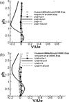 |
Fig. 14 Profile of the mean vertical velocity field after the obstacle for x = 4 h at the bottom of: (a) a water channel and (b) an air tunnel. |
3.2.2 Components of turbulence intensity field
Figures 15 and 16 illustrate the profiles of the horizontal and vertical turbulence intensity for the different inlet velocities for the water channel and the air tunnel. From the curves, it is observed that the turbulence intensity increases from the bottom wall of the channel to the upper limit of the obstacle, then it decreases for y > 1.5 h. In general, we mark that the turbulence intensity is maximal in the interval between y/h = 1 and y/h = 1.5, but it is almost zero on the walls of the water channel and the air tunnel. The horizontal and vertical turbulence intensities are clearly intensified for Figure 16b where the inlet velocity Ue2 = 2Ue1. In fact, for this curve, the production of turbulent energy is effected at the level of the fluid interface at different velocity where the shearing is very important. The high deformation rate in this region entails a relatively large production of turbulent energy.
 |
Fig. 15 Profile of horizontal turbulence intensity after the obstacle for x = 4 h at the bottom of: (a) a water channel and (b) an air tunnel. |
 |
Fig. 16 Profile of vertical turbulence intensity after the obstacle for x = 4 h at the bottom of: (a) a water channel and (b) an air tunnel. |
3.2.3 Reynolds shear stress
Figure 17 illustrates the profiles of the Reynolds shear stress for the different inlet velocities of the abscissa x = 4 h. The negativity of Reynolds shear stress indicates the recirculation zone. There is a big intensification in the case where Ue2 = 2Ue1 throughout the water channel and the air tunnel. And this results from the increase in absolute values of the two fields of vertical and horizontal velocity. The values of the Reynolds shear stress for the air tunnel are superior in terms of absolute value to those of the water channel given the difference in the Reynolds number Reh of shear flows [31].
 |
Fig. 17 Profile of Reynolds shear stress after the obstacle for x = 4 h at the bottom of: (a) a water channel and (b) an air tunnel. |
3.2.4 Scalar dispersion
Figure 18 shows the profiles of the mean scalar concentration for various inlet velocities of the abscissa x = 4 h. The mean scalar concentration is increasing after the obstacle with maximum values for the water channel higher than those for air tunnel given the difference in kinematic viscosity θ and the Reynolds number Reh.
This concentration is elevated on the interval y/h = [0,2] as well for the simulation of sheared flow with the velocity Ue2 = 2Ue1. It then decreases on the part above the obstacle until it becomes zero for the different velocities when y/h = 3. While for the last simulation, it remains positive until the upper limit of the domain.
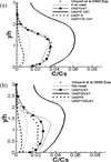 |
Fig. 18 Profile of the mean scalar concentration after the obstacle for x = 4 h at the bottom of: (a) a water channel and (b) an air tunnel. |
4 Conclusion
In this study, we simulated numerically, using the Fluent software; permanent and three-dimensional shear flows of two Newtonian fluids, around a cuboid obstacle at the bottom of a water canal and a tunnel of air. We presented first the fields of horizontal and vertical mean velocity; afterwards, horizontal and vertical turbulence intensity; then the Reynolds shear stress and finally, the mean scalar concentration. The positions located after the obstacle and encountered by a turbulent shear flow have shown in general a recirculation zone with a high concentration scalar; the regions at the boundary layer after the obstacle comprise a high turbulent energy. Thus the aim of this work was to explain the influence of inlet velocities on the parameters of shear flows. For the field of horizontal mean velocity, the maximal velocity values are obtained above the obstacle until the shear interface of the flow at inlet velocity Ue2 = 2Ue1. For the field of vertical mean velocity, it was found that the region admitting positive values and negative values becomes wider for the inlet velocity Ue2 = 2Ue1 in comparison with the other inlet velocities. Therefore this increase relates to the increase of the difference of the inlet velocities between the two fluids. The third variable to interpret is the turbulence intensity: Maximal values of the horizontal and vertical turbulence intensity are obtained for the inlet velocity Ue2 = 2Ue1 in the area downstream of the obstacle at 1.5 of its height. For the Reynolds shear stress, it was noticed that its values are negative due to the horizontal and vertical mean velocity field product. They are important for the inlet velocity Ue2 = 2Ue1 at the level of 1.5 of the height of the obstacle. For the scalar dispersion, the obtained curves have shown that, for all inlet velocities, the dispersion is carried out on the area downstream of the obstacle and remains low on the upper part of study area except for the inlet velocity Ue2 = 2Ue1, where it becomes more important by comparing it with other inlet velocities and this returns to the shearing of the fluid at the velocity Ue2 on the fluid at lower velocity Ue1. Thus, the production of energy will be more important at the boundary layer after obstacle where the shear is very strong. Indeed, the high deformation rate in this region entails, proportionally to inlet velocities, a large production of turbulent energy and an important scalar dispersion. The coupling between the use of hybrid grid and the turbulence model K–ε leads to better agreement with the experimental results of [8] to the water channel as well as the air tunnel. Therefore, the results of this study can be applied in various fields such as the extraction of energy, the orientation of the port infrastructure, the dispersion of pollutants flow in the boundary layers and the determination of the hydrodynamics of a coastal zone.
Nomenclature
C: dimensionless scalar concentration
H: height of the channel or tunnel (m)
h: height of the obstacle (m)
K: turbulent kinetic energy
L: length of the channel and tunnel (m)
l: width of the channel or tunnel (m)
P: pressure (bar)
 :
average pressure (bar)
:
average pressure (bar)
p′: pressure fluctuation
Reh: Reynolds number
Uτ: friction velocity
Ue: velocity inlet of the flow (m s−1)
 :
average velocity (m s−1)
:
average velocity (m s−1)
u′: velocity fluctuation
t: dimensionless time
x, y, z: Cartesian coordinates
Greek letters
ϵ: dissipation rate
μ: dynamic viscosity (kg m−1 s−1)
ϑ: kinematic viscosity (m2 s−1)
νt: turbulent viscosity
ρ: density (kg m−3)
σk: Prandtl number related to turbulent kinetic energy
σϵ: Prandtl number related to dissipation rate
δ: thickness of the boundary layer
τb: total wall shear stress
τs: local skin friction
η: height of the bedform
Superscript
′: dimensional variable
Subscripts
1, 2, 3: index of the Cartesian coefficient
References
- J.M. Tomas, M.J.B.M. Pourquie, H.J.J. Jonker, The influence of an obstacle on flow and pollutant dispersion in neutral and stable boundary layers, J. Atmos. Environ. 113 (2015) 236–246 [CrossRef] [Google Scholar]
- N.E. Mejia, Etude numérique du cisaillement des géomatériaux granulaires cohésifs: passage micro-macro, microstructure, et application à la modélisation de glissements de terrain, Thèse, Université Montpellier II, France, 2008 [Google Scholar]
- D.J. Korteweg, G. de Vries, On the change of form of long waves advancing in a rectangular canal, and on a new type of long stationary waves, Philos. Mag. 39 (1895) 422–443 [CrossRef] [MathSciNet] [Google Scholar]
- WAMDI Group, The WAM model – a third generation ocean wave prediction model, J. Phys. Oceanogr. 18 (1988) 1775–1810 [CrossRef] [Google Scholar]
- G.J. Komen, L. Cavaleri, M. Donelan, K. Hasselmann, S. Hasselmann, P.A.E.M. Janssen, Dynamics and modelling of ocean waves, Cambridge University Press, New York, 1994, pp. 275–296 [Google Scholar]
- A. Ouahsine, H. Smaoui, K. Meftah, P. Sergent, F. Sabatier, Numerical study of coastal sandbar migration by hydro-morphodynamical coupling, Environ. Fluid Mech. 13 (2012) 169–187 [CrossRef] [Google Scholar]
- L.C. Van Rijn et al., Transport of fine sands by currents and waves, J. Waterways Port Coastal Ocean Eng. ASCE 19 (1995) 1181–1189 [Google Scholar]
- J.Y. Vinçont, S. Simoens, M. Ayrault, M. Wallace, Passive scalar dispersion in a turbulent boundary layer from a line source at the wall and downstream of an obstacle, J. Fluid Mech. 424 (2000) 127–167 [CrossRef] [Google Scholar]
- R.N. Zare, My life with LIF: a personal account of developing laser-induced fluorescence, Annu. Rev. Anal. Chem. 5 (2012) 1–14 [Google Scholar]
- J. Frisvad, N. Christensen, H. Jensen, Computing the scattering properties of participating media using Lorenz-Mie theory, ACM Trans. Graph. 26 (2007) 51–60 [CrossRef] [Google Scholar]
- R. Rossi, G. Iaccarino, Numerical simulation of scalar dispersion downstream of a square obstacle using gradient-transport type models, J. Atmos. Environ. 43 (2009) 2518–2531 [CrossRef] [Google Scholar]
- H.K. Versteeg, W. Malalasekera, An introduction to computational fluid dynamics: the finite volume method, Pearson Education, England, 2007, pp. 30, 43–49 [Google Scholar]
- A. Amahmouj, E.M. Chaabelasri, N. Salhi, Computations of pollutant dispersion in coastal waters of Tangier's bay, Int. Rev. Model. Simulat. 5 (2012) 1588–1595 [Google Scholar]
- T. Watanabe, Y. Sakai, K. Nagata, Y. Ito, Large eddy simulation study of turbulent kinetic energy and scalar variance budgets and turbulent/non turbulent interface in planer jets, J. Fluid Dyn. Res. 84 (2016) 021407 [CrossRef] [Google Scholar]
- F.M. White, Viscous fluid flow, 3rd ed., McGraw-Hill, 2006, pp. 31, 43–49 [Google Scholar]
- R. Eymard, T.R. Gallouët, R. Herbin, The finite volume method, in: Handbook of Numerical Analysis, Vol. 7, North-Holland, Amsterdam 2000, pp. 713–1020 [Google Scholar]
- M. Hazewinkel (ed.), Seidel method, Encyclopedia of Mathematics, Springer, 2001, pp. 23, 517–527 [Google Scholar]
- D.M. David, M.R. Stephen, An embedded boundary Cartesian grid scheme for viscous flows using a new viscous wall boundary condition treatment, Presented at the AIAA 42nd Aerospace Sciences Meeting, AIAA Paper 0581, 2004 [Google Scholar]
- D.S. Jang, R. Jetli, S. Acharya, Comparison of the piso, simpler and simplec algorithm for the treatment of the pressure velocity coupling in steady flow problems, J. Numer. Heat Transfer 10 (1986) 209–228 [Google Scholar]
- C. Hirsch, Numerical computation of internal and external flows, Energy Convers. Manage. 44 (1999) 381–388 [Google Scholar]
- J.F. Straube, E.F.P. Burnett, Driving rain and masonry veneer, Water leakage through building facades, ASTM STP 1314, 2011 [Google Scholar]
- H.J. Hussein, R.J. Martinuzzi, Energy balance for turbulent flow around a surface mounted cube placed in a channel, Phys. Fluids 8 (1996) 764–780 [CrossRef] [Google Scholar]
- D. Spalding, A single formula for the law of the wall, J. Appl. Mech. 28 (1961) 455–458 [CrossRef] [Google Scholar]
- H. Smaoui, A. Ouahsine, Extension of the skin shear stress Li's relationship to the flat bed, Environ. Fluid Mech. 12 (2012) 201–207 [CrossRef] [Google Scholar]
- P.R. Spalart, Direct simulation of a turbulent boundary layer up to Rθ = 1410, J. Fluid Mech. 187 (1988) 61 [CrossRef] [Google Scholar]
- K. Cartwright, Determining the effective or RMS voltage of various waveforms without calculus, Technol. Interface 8 (2007) 1–20 [EDP Sciences] [Google Scholar]
- S.B. Pope, Turbulent flows, Cambridge University Press, UK, 2000 [CrossRef] [Google Scholar]
- G.G. Katul, D. Li, M. Chameki, E. Bou-Zeid, Mean scalar concentration profile in a sheared and thermally stratified atmospheric surface layer, Phys. Rev. 87 (2013) 023004 [Google Scholar]
- D.C. Wilcox, Formulation of the K-ω turbulence model revisited, AIAA J. 46 (2008) 2823–2838 [Google Scholar]
- B. Andersson, R. Andersson, Computational fluid dynamics for engineers, 1st ed., Cambridge University Press, New York, 2012, p. 97 [Google Scholar]
- W.F.F. Riley, L.D. Sturges, D.H. Morris, Mechanics of materials, 5th ed., John Wiley & Sons, New York, 1998, 720 pp. [Google Scholar]
Cite this article as: M. Toumi, S.H. Salah, W. Hassen, S. Marzouk, H.B. Aissia, J. Jay, Three-dimensional study of parallel shear flow around an obstacle in water channel and air tunnel, Mechanics & Industry 18, 505 (2017)
All Tables
All Figures
|
Fig. 1 Physical model of: (a) water channel and (b) air tunnel. |
| In the text | |
|
Fig. 2 (a) Hybrid mesh in 3D and (b) zoom on the obstacle. |
| In the text | |
|
Fig. 3 Mesh sensibility on the horizontal mean velocity field after the obstacle for x = 4 h at the bottom of (a) a water channel and (b) an air tunnel. |
| In the text | |
|
Fig. 4 Profile of mean velocity field without obstacle: (a) in the water channel and (b) in the air tunnel. |
| In the text | |
|
Fig. 5 Profile of Reynolds shear stress without obstacle: (a) in the water channel and (b) in the air tunnel. |
| In the text | |
|
Fig. 6 Contour of horizontal velocity field around the obstacle in the water channel (a–c), in the air tunnel (d–f) for models (a, d) RSM, (b, e) K–ω, and (c, f) K–ε. |
| In the text | |
|
Fig. 7 Profile of vertical average velocity field after the obstacle at the bottom of: (a) a water channel for x = 4 h, (b) for x = 6 h, (c) an air tunnel for x = 4 h, and (d) for x = 6 h. |
| In the text | |
|
Fig. 8 Profile of the turbulence intensity: (a) horizontal for x = 4 h, (b) x = 6 h, (c) vertical for x = 4 h, (d) x = 6 h; after the obstacle at the bottom of a water channel. |
| In the text | |
|
Fig. 9 Profile of the turbulence intensity: (a) horizontal for x = 4 h, (b) x = 6 h, (c) vertical for x = 4 h, (d) x = 6 h; after the obstacle at the bottom of an air tunnel. |
| In the text | |
|
Fig. 10 Profile of Reynolds shear stress after the obstacle at the bottom of: (a) a water channel for x = 4 h, (b) x = 6 h, (c) an air tunnel for x = 4 h, (d) x = 6 h. |
| In the text | |
|
Fig. 11 Profile of the mean scalar concentration after the obstacle at the bottom of: (a) a water channel for x = 4 h, (b) x = 6 h, (c) an air tunnel for x = 4 h, (d) x = 6 h. |
| In the text | |
|
Fig. 12 Profile of the mean horizontal velocity field after the obstacle: (a) at the bottom of a water channel for x = 4 h, (b) for x = 6 h, (c) at the bottom of an air tunnel x = 4 h, (d) x = 6 h. |
| In the text | |
|
Fig. 13 Profile of the mean horizontal velocity field after the obstacle for x = 4 h at the bottom of: (a) a water channel and (b) an air tunnel. |
| In the text | |
|
Fig. 14 Profile of the mean vertical velocity field after the obstacle for x = 4 h at the bottom of: (a) a water channel and (b) an air tunnel. |
| In the text | |
|
Fig. 15 Profile of horizontal turbulence intensity after the obstacle for x = 4 h at the bottom of: (a) a water channel and (b) an air tunnel. |
| In the text | |
|
Fig. 16 Profile of vertical turbulence intensity after the obstacle for x = 4 h at the bottom of: (a) a water channel and (b) an air tunnel. |
| In the text | |
|
Fig. 17 Profile of Reynolds shear stress after the obstacle for x = 4 h at the bottom of: (a) a water channel and (b) an air tunnel. |
| In the text | |
|
Fig. 18 Profile of the mean scalar concentration after the obstacle for x = 4 h at the bottom of: (a) a water channel and (b) an air tunnel. |
| In the text | |
Current usage metrics show cumulative count of Article Views (full-text article views including HTML views, PDF and ePub downloads, according to the available data) and Abstracts Views on Vision4Press platform.
Data correspond to usage on the plateform after 2015. The current usage metrics is available 48-96 hours after online publication and is updated daily on week days.
Initial download of the metrics may take a while.