| Issue |
Mechanics & Industry
Volume 21, Number 5, 2020
Scientific challenges and industrial applications in mechanical engineering
|
|
|---|---|---|
| Article Number | 509 | |
| Number of page(s) | 10 | |
| DOI | https://doi.org/10.1051/meca/2020032 | |
| Published online | 10 August 2020 | |
Regular Article
Identification of the pore size distribution of a porous medium by yield stress fluids using Herschel-Bulkley model
1
Laboratoire de l’Ingénierie et Technologies Appliquées, Ecole Supérieure de Technologie, Université Sultan Moulay Slimane,
Béni Mellal,
Morocco
2
LAMPA, Ecole Nationale Supérieure d’Arts et Métiers, 2 Boulevard du Ronceray,
49035
Angers Cedex 01,
France
* e-mail: This email address is being protected from spambots. You need JavaScript enabled to view it.
Received:
13
October
2019
Accepted:
3
April
2020
Abstract
In this paper, we present a new method to determine the pore-size distribution (PSD) in a porous medium. This innovative technique uses the rheological properties of non-Newtonian yield stress fluids flowing through the porous sample. In a first approach, the capillary bundle model will be used. The PSD is obtained from the measurement of the total flow rate of fluid as a function of the imposed pressure gradient magnitude. The mathematical processing of the experimental data, which depends on the type of yield stress fluid, provides an overview of the pore size distribution of the porous material. The technique proposed here was successfully tested analytically and numerically for usual pore size distributions such as the Gaussian mono and multimodal distributions. The study was conducted for yield stress fluids obeying the classical Bingham model and extended to the more realistic Herschel-Bulkley model. Unlike other complex methods, expensive and sometimes toxic, this technique presents a lower cost, requires simple measurements and is easy to interpret. This new method could become in the future an alternative, non-toxic and cheap method for the characterization of porous materials.
Key words: Porous material / pore-size distribution / non-Newtonian yield stress fluid / Herschel-Bulkley model / fractional derivative / numerical inversion
© A. Oukhlef et al., published by EDP Sciences 2020
 This is an Open Access article distributed under the terms of the Creative Commons Attribution License (http://creativecommons.org/licenses/by/4.0), which permits unrestricted use, distribution, and reproduction in any medium, provided the original work is properly cited.
1 Introduction
Porous media are found almost everywhere around us [1–4], whether in living matter (human skin, cartilage, bone, etc.), inert matter (soils, layers sedimentary rocks, etc.) or industrial materials (concretes, cements, powders, textiles, etc.). The characterization of porous media in terms of porosity, specific surface, PSD etc., is an important issue for many industrial sectors: assisted petroleum recovery, thermal insulation of buildings, CO2 sequestration, energy storage, etc. The phenomena related to flow through porous media have occupied and continue to stimulate a strong research activity, both fundamental and applied. The main objective of this work is to propose a new non-polluting, simple and economic method to determine the pore size distribution of a porous medium without the defects of the currently existing techniques. Among them, we can cite classical methods such as: (i) the mercury intrusion porosimetry (MIP) [1–3,5]. This technique is based on the existence of a threshold below which the pores cannot be invaded. Indeed, due to its large surface tension mercury does not wet most materials. A pressure difference ΔPlg must be imposed so that mercury penetrates the pores whose radii rp are greater than  where σlg is the liquid/gas interfacial tension and θ the contact angle. Because of the harmful effects of mercury vapor, this technique is destined to be abandoned; (ii) the method of isothermal gas adsorption [6], based on the molecular Van der Waals interactions between a condensing vapor and the internal surface of the pores is particularly adapted to the characterization of porous media with mesopores (in the range 5 nm ≤ r ≤ 100 nm). There are other alternative techniques that can characterize the PSD like thermoporometry [7], the Small Angle Neutron (SANS) or X-Ray Scattering (SAXS) [8,9], nuclear magnetic resonance (NMR) [10], not to mention the destructive methods such as stereological analysis of polished slices [11]. All these techniques are either difficult to implement or expensive (microscopy, image acquisition by X-ray Computerized Micro-Tomography, etc.). The above cited classical methods are based on the existence of a threshold below which the pores cannot be invaded according to a thermodynamic control parameter. Like the aforementioned techniques, our new approach is based on the injection of non-Newtonian yield stress fluid into the porous medium (invasive method). In the present method, we propose to use the rheological properties of yield stress fluid to scan different pore scales and determine the PSD. The basic idea is the following: in order to set such fluids into motion, it is necessary to impose between both ends of a pore a pressure gradient whose magnitude
  is greater than a critical value depending on the fluid yield stress
  and the pore radius
  . In other words, for a given pressure gradient magnitude ∇P, only the pores whose radius is greater than the critical radius r0 = 2τ0∕∇P are invaded. Then it is possible to scan the PSD by adjusting the pressure gradient step by step and measuring the corresponding flow rate Q. From the curve Q = f(∇P), it is possible to extract the PSD solving an inverse problem. This technique has been successfully tested on unimodal, bi or tri-modal Gaussian PSD. The problem inversion depending on the rheological behavior of the fluid, we started using ideal yield stress fluids such as Bingham fluids [12]. Since it is rather difficult to find fluids obeying these rheological laws, we have generalized our method to the Herschel-Bulkley model [13] which better describes most of the non-Newtonian yield stress fluids. In this work, we will give the results of this generalized model by presenting first the analytical expression of the solution of the inverse problem coming from the resolution of the associated integral equation described below. So, we can calculate the probability density depending on the partial derivatives (integer or fractional) of the characteristic curve (Q =f(∇P)). This paper also reports an improvement to this technique: the solution of the problem for the PSD identification using a method based on a numerical approach with yield stress fluids such as Herschel-Bulkley model.
2 Models and procedure
2.1 Formulation of the problem and solution
In this paper, the porous material is described by a bundle of capillary tubes [14,15], the radii of which are distributed according to an unknown probability density function p(r). This model,originally introduced by Purcell [16], is used nearly in all theoretical studies of porous media because of its amenability to analytical treatment and because variables that are difficult or impossible to measure physically can be computed directly from this model. Still, let us review the main limitations of this model:
-
The first one concerns the maximum porosity: for a porous medium whose pores have the same radius, the maximum 2D-packing is the hexagonal packing arrangement with a maximum porosity of
 in an infinite medium (this value decreases when the confinement increases and strongly depends on the shape of the boundaries). The maximum porosity for a random close packing of disks is even lesser with a maximal value
ϕ = 0.84 for an infinite medium. These analytical values overestimate the maximal porosity because the contact of the pores would not be possible in a “real” capillary bundle porous medium in which some solid material has to remain between the pores in order to guarantee the structural robustness of the material. Some values around
ϕ = 0.78 are considered acceptable in practice. Moreover, let us note that this model gives access only to the open porosity since it is based on the flow properties;
in an infinite medium (this value decreases when the confinement increases and strongly depends on the shape of the boundaries). The maximum porosity for a random close packing of disks is even lesser with a maximal value
ϕ = 0.84 for an infinite medium. These analytical values overestimate the maximal porosity because the contact of the pores would not be possible in a “real” capillary bundle porous medium in which some solid material has to remain between the pores in order to guarantee the structural robustness of the material. Some values around
ϕ = 0.78 are considered acceptable in practice. Moreover, let us note that this model gives access only to the open porosity since it is based on the flow properties; -
It neglects complex features of porous media such as tortuosity, the dead arms and it neglects interconnectivity between pores as it assumes unidirectional flow;
-
The contraction-expansion features of non-Newtonian yield stress fluid flows cannot be accounted for because this model assumes a single radius along each pore of the bundle with no variation in the cross-sectional area;
-
It cannot be representative for flows in an anisotropic medium due to its assumption of unique permeability along propagation direction;
-
It neglects the elongation effects associated with porous media flows.
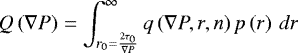
However, some of the limitations cited above can be erased by more complex variants not considered here. In our study, we ignore the tortuosity that only affects the characteristic curve by increasing the length of the pores [1,2] and not the non-dimensional PSD. We will use this model to derive the inversion technique which allows us to obtain the PSD from the characteristic curve for a given yield stress fluid in non-inertial regimes. Under these conditions, the expression of the total flow rate Q through this capillary model, when a pressure gradient magnitude ∇P is imposed on this system, is a function of the elementary flow rate q(∇P, r, n) in each capillary and of the probability density p(r):
 (1)
(1)
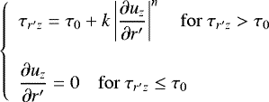
In this study, our goal is to extract the probability density p(r) from the curve describing the evolution of total flow rate Q(∇P) as a function of the pressure gradient magnitude of a Herschel-Bulkley fluid (H-B) through a porous medium. This measured flow rate is calculated directly from the integral equation (1) when p(r) is known. If this distribution is unknown, this relation constitutes a Volterra equation of the first kind, whose kernel q(∇P, r, n) is the elementary flow rate in each capillary and Q(∇P) constitutes the source term obtained experimentally. The kernel q(∇P, r, n) depends on the yield stress fluid type and the Herschel-Bulkley model is used here because it describes the rheological behavior of most non-Newtonian yield stress fluids more realistically than the Bingham model. Indeed, the H-B model can take into account the pseudo-plastic or dilatant behavior of the real yield stress fluids and constitute a generalization of the Bingham model. In H-B fluids beyond the yield stress τ0, the linearity of the shear stress with the shear rate is replaced by a power law. It is, therefore, a model with three parameters: the yield stress τ0, the consistency of the fluid k and power-law index n. The rheological behavior law describing this model is given by:
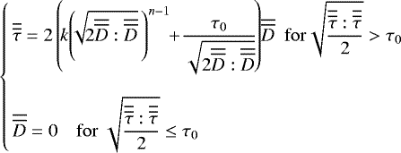 (2)
(2)
with  the shear stress tensor and
  the rate of deformation tensor. For the flow in a tube with circular cross-section, these equations take the simpler form:
 (3)
(3)
where  is the shear stress,
  the rate of deformation and r′ is the radial coordinate. The elementary flow rate of the Herschel-Bulkley fluid through a capillary of circular cross-section with radius r, which constitutes the kernel of equation (1), is given by [17]:
![Mathematical equation: \begin{align*}&q\left(\nabla{P},r,n\right)\nonumber\\ &\hskip-3pt =\!\left\{\begin{array}{l} \displaystyle n\pi_{}r^{3}\left(\frac{r\nabla{P}}{2k}\right)^{\frac{1}{n}}\left(1-\frac{r_{0}}{r}\right)^{\frac{n+1}{n}}\vspace{0.2cm}\\ \hspace{0.5cm} \displaystyle \left[\frac{\left(1-\frac{r_{0}}{r}\right)^{2}}{\left(3n+1\right)}+\frac{\frac{2r_{0}}{r}\left(1-\frac{r_{0}}{r}\right)}{\left(2n+1\right)}+\frac{\left(\frac{r_{0}}{r}\right)^{2}}{\left(n+1\right)}\right] \ {\rm{for}}\ r>r_{0} \\ \\ \displaystyle 0 \ {\rm{for}}\ r\leq{r_{0}} \end{array}\right. \end{align*}](/articles/meca/full_html/2020/05/mi190324/mi190324-eq13.png) (4)
(4)
For r ≤ r0 the fluid does not flow. The critical radius r0 = 2τ0∕∇P is also the radius of the core zone of the plug flow. The pore size distribution  can be obtained through differential operators applied to
  [13]:
[13]:
![Mathematical equation: \begin{align*}p\left(r\right)=&\,\displaystyle\frac{2^{\left(1+3n\right)/n}k^{1/n}\left(\nabla{P}\right)^{2}}{16\pi\tau_{0}r^{\left(1+3n\right)/n}\left(1/n\right)!}\left[\left(\frac{1+4n}{n}\right)\frac{\partial^{\left(1+n\right)/n} .}{\partial \left(\nabla{P}\right)^{\left(1+n\right)/n}}\right.\nonumber\\ & +\displaystyle \left.\nabla{P}\frac{\partial^{\left(1+2n\right)/n} .}{\partial \left(\nabla{P}\right)^{\left(1+2n\right)/n}}\right]Q~|_{\nabla{P}=\frac{2\tau_{0}}{r}} \end{align*}](/articles/meca/full_html/2020/05/mi190324/mi190324-eq16.png) (5)
(5)
It should be noted (i) that equation (5) is valid only for  but since the rational numbers are a dense subset of the real numbers, any real number has rational numbers arbitrarily close to it and (ii) that for n = 1 the Herschel-Bulkley model reduces to that of Bingham fluid and equation (5) reduces to that obtained by Ambari et al. [18] and (iii) that in equation (5), (1∕n)! is finite even for any real value of n≠0 and is calculated by the Gamma function:
![Mathematical equation: \[ \displaystyle \left(\frac{1}{n}\right)!=\UpGamma\left(1+\frac{1}{n}\right)=\int_{0}^{\infty} e^{-x}x^{1/n}dx \]](/articles/meca/full_html/2020/05/mi190324/mi190324-eq18.png)
2.2 Analytical inverse method to determine the PSD
In the case where the power-law index is n = 1∕q with  , a general relationship is obtained between the probability density p(r) and the integer partial derivatives of the total flow
  . In the case where q is non-integer it is possible to generalize this formula considering these derivatives as fractional. This will be justified later. In order to reduce the number of physical parameters involved in this problem, we will normalize the previous equations, using as characteristic scales L for the length and τ0 ∕L for the pressure gradient magnitude where L is the thickness of the studied sample (directly accessible) and not the mean radius of the capillaries which is still unknown and would require a complementary measurement. Therefore, the non-dimensional kernel is then given by:
![Mathematical equation: \begin{align*}&q^{+}\left(\nabla{P}^{+},r^{+},n\right)\nonumber\\ &\hskip-3pt =\! \left\{\begin{array}{l} He^{H-B}\frac{1}{2^{\frac{1}{n}}}\left(\frac{1}{2n+1}\right)\frac{1}{\left(\nabla{P}^{+}\right)^{3}}\left(r^{+}\nabla{P}^{+}-2\right)^{1+\frac{1}{n}}\vspace{0.2cm}\\ \hspace{0.5cm} \displaystyle \left[8n^{2}+4n\left(n+1\right)r^{+}\nabla{P}^{+}\right.\vspace{0.2cm}\\ \hspace{1cm} +\displaystyle \left. \left(2n^{2}+3n+1\right)\left(r^{+}\nabla{P}^{+}\right)^{2} \right] \ {\rm{for}}\ r^{+}>r^{+}_{0} \\ \\ \displaystyle 0 \ {\rm{for}}\ r^{+}\leq{r^{+}_{0}} \end{array}\right. \end{align*}](/articles/meca/full_html/2020/05/mi190324/mi190324-eq21.png) (6)
(6)
with 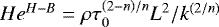 the Hedström number in the case of a Herschel Bulkley fluid [19], ρ the density of fluid and
  the non-dimensional critical radius. In equation (6), the flow rate is normalized by the characteristic flow rate:
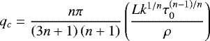 (7)
(7)
Figure 1 below presents the evolution of the elementary flow rate q+ (that is to say the kernel of Eq. (1)) in a pore of radius r+ =1 as a function of the imposed pressure gradient magnitude ∇P+ for different power-law index and for a Hedström number HeH−B = 0.02.
As for non-dimensional pore size distribution:
![Mathematical equation: \begin{align*}\hskip-11pt p^{+}\left(r^{+}\right) &=\displaystyle \frac{n\left(\nabla{P}^{+}\right)^{\left(1+5n\right)/n}}{16He^{H-B}\left(3n+1\right)\left(1+n\right)\left(1/n\right)!}\nonumber\\ \displaystyle &\quad\left[\left(\frac{1+4n}{n}\right)\frac{\partial^{\left(1+n\right)/n} .}{\partial \left(\nabla{P}^{+}\right)^{\left(1+n\right)/n}}\right.\nonumber\\ &\quad+\displaystyle \left.\nabla{P}^{+}\frac{\partial^{\left(1+2n\right)/n} .}{\partial \left(\nabla{P}^{+}\right)^{\left(1+2n\right)/n}}\right]Q^{+}~|_{\nabla{P}^{+}=\frac{2}{r^{+}}} \end{align*}](/articles/meca/full_html/2020/05/mi190324/mi190324-eq25.png) (8)
(8)
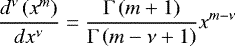
In the case, where n is non-integer, the calculation of the fractional derivatives in equation (8) are very difficult unless the derived function is simple. One of the simplest solutions for non-integer derivation is when the derived function is a polynomial. it can be carried out by means of the following relation defined by Riemann [20]:
 (9)
(9)
where ν is the non-integer derivation order, Γ the gamma function and m the order of the derivative of a monomial, with (x = ∇P). In our study, the above relation will be used to calculate the different fractional derivatives that occur in equation (8) provided a polynomial fit of the evolution  is given (in the present study, all the characteristic curves
  were fitted by polynomial functions of maximum order 40 because this order leads to a satisfactory inversion of all the curves whatever the value of the power-law index n. However, we have noticed that the lower the value of n, the lower the order of the polynomials to use. For instance, for n = 0.9, a polynomial of order 15 starts to give satisfactory results). Remember that in the case where n = 1∕q with
  , the two successive derivatives are integers. In all cases, the distribution will be calculated by using equation (8). In the next section we explain the approach followed to obtain this inverse distribution.
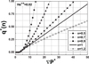 |
Fig. 1 Elementary flow rate vs. pressure gradient magnitude for different power-law index and HeH−B = 0.02. |
2.2.1 Inversion in the case of a Bingham fluid (n = 1)
As a first attempt to test this method, let us assume that the fluid is a Bingham fluid (n = 1) and that the PSD is of Gaussian type of mean radius μ and standard deviation σ. Written in non-dimensional form (r+ = r∕L, μ+ = μ∕L, σ+ = σ∕L and  ), this distribution is:
![Mathematical equation: \begin{equation*}p^{+}\left(r^{+}\right)=\frac{1}{\sigma^{+}\sqrt{2\pi}}\exp\left[-\frac{\left(r^{+}-\mu^{+}\right)^{2}}{2{\sigma^{+}}^{2}}\right] \end{equation*}](/articles/meca/full_html/2020/05/mi190324/mi190324-eq31.png) (10)
(10)
and the normalized Volterra equation (Eq. (1)) is:
 (11)
(11)
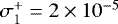
Using equations (6), (10) and (11), it is possible to calculate the characteristic curve  . In Figure 2 above, it is shown for μ+ = 10−4, σ+ = 2 × 10⁻⁵ and HeH−B = 0.02. This figure shows the non-dimensional total flow rate vs. the non-dimensional pressure gradient magnitude resulting from the flow of the Bingham fluid through such a porous medium. This figure is characterized by a first region at low pressure gradients in which the flow rate is zero. This region extends until the largest pore in the material is invaded. It is followed by a second region in which the flow rate increases with the pressure gradient. Now, let us start from this characteristic curve
  and let us try to calculate
  . For n = 1, equation (8) becomes:
![Mathematical equation: \begin{align*}\displaystyle p^{+}\left(r^{+}\right)=&\,\frac{\left(\nabla{P}^{+}\right)^{6}}{128He^{H-B}}\left[5\frac{\partial^{2} .}{\partial \left(\nabla{P}^{+}\right)^{2}}+\nabla{P}^{+}\frac{\partial^{3} .}{\partial \left(\nabla{P}^{+}\right)^{3}}\right]\nonumber\\ &\times\,Q^{+}~|_{\nabla{P}^{+}=\frac{2}{r^{+}}} \end{align*}](/articles/meca/full_html/2020/05/mi190324/mi190324-eq36.png) (12)
(12)
Because equation (12) has only integer derivatives, it can be directly applied to the non-dimensional characteristic curve (Fig. 2) to calculate  . It is plotted in Figure 3 together with the original normal distribution (Eq. (10)) and the agreement between both curves is very good (see the article [12]).
We have also tried to use the method involving the polynomial fit of the characteristic curve  and its fractional derivatives (Eq. (9)). The results obtained by this method are shown in Figure 4. It shows that this technique is also relevant even though it introduces some noise for the small radii related to the polynomial fit needed here.
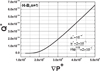 |
Fig. 2 Total flow rate vs. pressure gradient magnitude for a Gaussian distribution and a Bingham fluid for HeH−B = 0.02. |
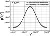 |
Fig. 3 Comparison between the initial and the analytically calculated PSD for a Bingham fluid. |
 |
Fig. 4 Comparison between the initial and the fractional method calculated PSD for a Bingham fluid. |
2.2.2 Inversion in the case of a Herschel-Bulkley fluid for n = 1/q with 
As a second attempt to test this method, let us make the problem more complex and consider a Herschel-Bulkley pseudo-plastic fluid whose power law index has the form n = 1∕q with  . In this case, the inversion procedure also involves integer partial derivatives of order 1 + q and 2 + q. For instance for n = 1∕2, the normalized PSD (Eq. (8)) writes as:
![Mathematical equation: \begin{align*}\displaystyle p^{+}\left(r^{+}\right)=&\,\frac{\left(\nabla{P}^{+}\right)^{7}}{240He^{H-B}}\left[6\frac{\partial^{3} .}{\partial \left(\nabla{P}^{+}\right)^{3}}+\nabla{P}^{+}\frac{\partial^{4} .}{\partial \left(\nabla{P}^{+}\right)^{4}}\right]\nonumber\\ &\times\,Q^{+}~|_{\nabla{P}^{+}=\frac{2}{r^{+}}} \end{align*}](/articles/meca/full_html/2020/05/mi190324/mi190324-eq40.png) (13)
(13)
Following the same procedure as in the previous section and for the same initial Gaussian distribution, we have calculated the characteristic curve  presented in Figure 5. Now, when equation (13) is applied to the characteristic curve (Fig. 5), the initially injected Gaussian PSD is retrieved as we can see in Figure 6. Likewise this distribution can be obtained using the fractional derivatives method (Fig. 7) with some additional noise for the smallest radii because of the poor description of the characteristic curve by the polynomial function when r is small.
 |
Fig. 5 Total flow rate vs. pressure gradient magnitude for a Gaussian distribution and a Herschel-Bulkley fluid for n = 1∕2 and HeH−B = 0.02. |
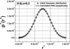 |
Fig. 6 Comparison between the initial and the analytically calculated PSD for a Herschel-Bulkley fluid with n = 0.5. |
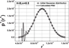 |
Fig. 7 Comparison between the initial and the fractional method calculated PSD for a Herschel-Bulkley fluid with n = 0.5. |
2.2.3 Inversion in the case of a Herschel-Bulkley fluid for n = p∕q with  \{1} and with
In the case where the flow index of the fluid is a rational number whose numerator is different from unity, the identification formula (Eq. (8)) presents also non-integer derivatives. In this case, only the fractional derivatives method is usable based on the polynomial fit of the characteristic curve. The results for a pseudo-plastic fluid (n = 0.9) are presented inFigures 8 and 9 for a normal distribution whose parameters are again μ+ = 10−4, σ+ = 2 × 10⁻⁵ and for HeH−B = 0.02. Likewise for the same set of parameters, the results concerning a dilatant fluid (n = 1.2) are given in Figures 10 and 11. We note that the inverse distribution can be obtained by the method using the fractional derivatives but like in the case of a Bingham fluid, some fluctuations appear for the small radii due to the lack of precision of the polynomial fit used here. Therefore, we will present in the next section another numerical method effective and robust and that can be applied to all yield stress fluids such as the Herschel-Bulkley fluids and for all kinds of distributions.
Note that this approach, based on the fractional derivatives and the polynomial interpolation function, fails for more complex distributions (bimodal or tri-modal) probably because of the unsuited interpolation function used here. This has motivated another numerical method based on the numerical discretization of the Volterra equation.
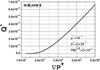 |
Fig. 8 Total flow rate vs. pressure gradient magnitude for a Gaussian distribution and a Herschel-Bulkley fluid for n = 0.9. |
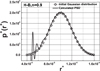 |
Fig. 9 Comparison between the initial and the fractional method calculated PSD for a Herschel-Bulkley fluid with n = 0.9. |
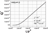 |
Fig. 10 Total flow rate vs. pressure gradient magnitude for a Gaussian distribution and a Herschel-Bulkley fluid for n = 1.2. |
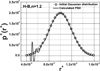 |
Fig. 11 Comparison between the initial and the fractional method calculated PSD for a Herschel-Bulkley fluid with n = 1.2. |
2.3 Numerical inverse method for determining PSD
An alternative method to solve the Volterra equation (Eq. (1)) is to use a matrix system. For this, we adopt the following approach: the pressure gradient magnitude (j-index) and the pore radius (i-index) are discretized using N points so that the source term  , the kernel
  and the PSD p(r) become respectively Qj = Qj(∇Pj), qij = q(∇Pj, ri, n) and pi = p(ri). The Volterra equation is then rewritten as follows:
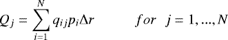 (14)
(14)
with Δr = (rmax − rmin)∕(N − 1). Mathematically, if the kernel qij is not singular, equation (14) has a unique solution which is given by the following relation:
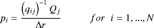 (15)
(15)
where  is the inverse matrix of the kernel.
2.3.1 Numerical approach
The non-dimensional form of the functions is used to solve the previous system. For this, we use the kernel in the form written in equation (6). This kernel is discretized using a non-dimensional radius step Δr+ and a non-dimensional pressure gradient magnitude step  such that:
![Mathematical equation: \[ \displaystyle \UpDelta{r^{+}}=(r_{\textrm{max}}^{+}-r_{\textrm{min}}^{+})/(N-1) \]](/articles/meca/full_html/2020/05/mi190324/mi190324-eq48.png)
![Mathematical equation: \[ \UpDelta{\left(\nabla{P}\right)^{+}}=(\nabla{P}_{\textrm{max}}^{+}-\nabla{P}_{\textrm{min}}^{+})/(N-1) \]](/articles/meca/full_html/2020/05/mi190324/mi190324-eq49.png)
with  and
and  for given values of
  and
and  . The discretized non-dimensional radius and pressure gradient magnitude now become:
![Mathematical equation: \[ \displaystyle r_{i}^{+}=r_{\textrm{min}}^{+}+\left(i-1\right)\UpDelta{r^{+}} \hspace{1cm} \displaystyle for \hspace{0.2cm} i=1,...,N \]](/articles/meca/full_html/2020/05/mi190324/mi190324-eq54.png)
![Mathematical equation: \[ \displaystyle \nabla{P}_{j}^{+}=\nabla{P}_{\textrm{min}}^{+}+\left(j-1\right)\UpDelta{\left(\nabla{P}\right)^{+}} \hspace{0.5cm} \displaystyle for \hspace{0.2cm} j=1,...,N \]](/articles/meca/full_html/2020/05/mi190324/mi190324-eq55.png)
The kernel matrix is then built with the previously discretized elements:
![Mathematical equation: \[ q_{ij}^{+}=q^{+}\left(\nabla{P}_{j}^{+},r_{i}^{+},n\right) \]](/articles/meca/full_html/2020/05/mi190324/mi190324-eq56.png)
with
![Mathematical equation: \begin{align*}q^{+}\left(\nabla{P}_{j}^{+},r_{i}^{+},n\right)=&\,He^{H-B}\frac{1}{2^{\frac{1}{n}}}\left(\frac{1}{2n+1}\right)\frac{1}{\left(\nabla{P}_{j}^{+}\right)^{3}}\\ &\times\,\left(r_{i}^{+}\nabla{P}_{j}^{+}-2\right)^{1+\frac{1}{n}}\\ &\times\displaystyle \left[\vphantom{\left(2n^{2}+3n+1\right)\left(r_{i}^{+}\nabla{P}_{j}^{+}\right)^{2}}8n^{2}+4n\left(n+1\right)r_{i}^{+}\nabla{P}_{j}^{+}\right.\\ & +\displaystyle \left. \left(2n^{2}+3n+1\right)\left(r_{i}^{+}\nabla{P}_{j}^{+}\right)^{2} \right] \end{align*}](/articles/meca/full_html/2020/05/mi190324/mi190324-eq57.png)
At this point, after having experimentally obtained the N components of the source vector Qj and calculated the inverse of the kernel matrix  , we can determine the unknown distribution pi. The number of values used (here N = 1000) can naturally be reduced depending on the desired accuracy. Indeed, to numerically invert the Volterra equation, we no longer need a large number of values as previously required in the case of the analytical and fractional derivatives methods. Note that in an experimental work, this is the number of points of the pressure gradient (or flow rate) that would command the number of points for the radius. But within the range of pressure gradients experimentally explored, if one wishes a finer discretization for the radius, it is always possible to interpolate the missing data of the pressure gradient (or the flow rate) in order to find a square matrix.
2.3.2 Numerical inversions of some distributions by using Herschel-Bulkley model
-
Herschel-Bulkley fluid with n = 1 (Bingham model)
As in most experiments it is cumbersome to obtain a large sample of data, we have tested the accuracy of the present numerical method on a sample of N = 25 points (instead of 1000 points used in the two previous methods). Figure 12 shows the characteristic curve for a normal distribution (μ+= 10−4, σ+ = 2 × 10⁻⁵) and a Bingham fluid (n = 1) for HeH−B = 0.02 and Figure 13 presents the results obtained by the numerical method compared to the initial Gaussian PSD. A good agreement is found here although the size of the sample is small which seems to be encouraging.
To verify the efficiency of this numerical technique with more complex distributions, a bimodal Gaussian distribution is considered, with two peaks at  and
and  and two different standard deviations
  and
and  . For a Bingham fluid (n = 1) at HeH−B = 0.02, the characteristic curve can be evaluated (Fig. 14). For this example, N = 1000 points are used to increase the accuracy.
Once again, when the numerical method is applied to the data in Figure 14, the initial bimodal Gaussian distribution is perfectly found (Fig. 15).
-
Herschel-Bulkley fluid with n = 0.9 (pseudo-plastic) and n = 1.2 (dilatant)
Finally, we can test this method on pseudo-plastic or dilatant yield stress fluids. Let us recall that these two cases generally require the use of the fractional derivatives method leading to some noise when the pore radius becomes very small. The two fluids tested here are characterized by the following parameters: HeH−B = 0.02, n =0.9 (pseudo-plastic) and n =1.2 (dilatant). A tri-modal Gaussian distribution is tested with  ,
,  ,
,  ,
,  ,
,  and
and  .
.
Figures 16 and 17 validate the pseudo-plastic case (n = 0.9) and Figures 18 and 19 validate the dilatant case (n = 1.2). Therefore, this numerical method seems very effective and robust and can be applied to all kind of yield stress fluids such as the Herschel-Bulkley for any power-law index n < 1 (pseudo-plastic behavior) orn > 1 (dilatant behavior) and for all kinds of distributions. All these tests show that the numerical inversion method is relevant for determining the pore size distribution p(r) provided that a sufficient number of points and well-adapted radius and pressure gradient magnitude intervals are taken.
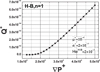 |
Fig. 12 Total flow rate vs. pressure gradient magnitude for a Gaussian distribution and a Bingham fluid (N = 25). |
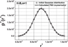 |
Fig. 13 Comparison between the initial and the numerically calculated PSD for a Bingham model with N = 25. |
 |
Fig. 14 Total flow rate vs. pressure gradient magnitude for a bimodal distribution ( |


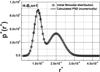 |
Fig. 15 Comparison between the initial and the numerically calculated PSD for a bimodal distribution ( |


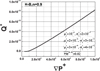 |
Fig. 16 Total flow rate vs. pressure gradient magnitude for a tri-modal distribution with ( |


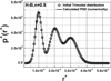 |
Fig. 17 Comparison between the initial and the numerically calculated PSD for a tri-modal distribution ( |


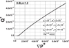 |
Fig. 18 Total flow rate vs. pressure gradient magnitude for a tri-modal distribution ( |


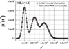 |
Fig. 19 Comparison between the initial and the numerically calculated PSD for a tri-modal distribution ( |


3 Conclusion
This work presents a new method for determining and identifying the pore size distribution of porous materials. It is based on the capillary bundle model like most of the other experimental techniques. This method uses non-Newtonian yield stress fluids. The existence of a yield stress gives the possibility to scan the pore distribution. Analytically, the total flow rate of such fluids into a porous medium appears as a Volterra integral equation of the first kind whose kernel is analytically known in the case of the flow into a straight capillary. The mathematical determination of the probability density p(r) function is possible using the partial derivatives (of integer or non-integer order) of the total flow rate of fluid through the porous medium as a function of the pressure gradient magnitude or by a numerical method based on the inverse matrix of the kernel. These techniques are successfully tested for Herschel-Bulkley fluids in the case of mono, bi or tri-modal Gaussian distributions but any other distribution or yield stress fluid (Casson, Robertson-Stiff, etc.) could be used potentially. However, in some cases the resolution of the Volterra equation should be done numerically and not analytically. We hope that this method could become in the future an alternative to the toxic and expensive existing methods for the characterization of porous materials.
References
- F.A.L. Dullien, Porous media – Fluid transport and pore structure, 2nd edn. Academic Press, Cambridge, 1992 [Google Scholar]
- A.E. Scheidegger, The physics of flow through porous media, 3rd edn., University of Toronto Press, Toronto, 1974 [Google Scholar]
- M. Kaviany, Principles of heat transfert in porous media, 2nd edn., Springer, Berlin, 1995 [Google Scholar]
- P.M. Adler, Porous media: geometry and transports, Butterworth-Heinemann, Oxford, 1992 [Google Scholar]
- Z.E. Heinemann, Fluid flow in porous media, Textbook series 1, 2003 [Google Scholar]
- E.P. Barrett, L.G. Joyner, P.P. Halenda, The determination of pore volume and area distributions in porous substances. Computations from Nitrogen isotherms, J. Am. Chem. Soc. 73, 373–380 (1951) [Google Scholar]
- M. Brun, A. Lallemand, J.-F. Quinson, C. Eyraud, A new method for the simultaneous determination of the size and the shape of pores: the thermoporometry, Thermochim. Acta 21, 59–88 (1977) [Google Scholar]
- H. Tamon, H. Ishizaka, Saxs study on gelation process in preparation of resorcinol-formaldehyde aerogel, J. Colloid Interface Sci. 206, 577–582 (1998) [Google Scholar]
- D. Pearson, A.J. Allen, A study of ultrafine porosity in hydrated cements using small angle neutron scattering, J. Mater. Sci. 20, 303–315 (1985) [Google Scholar]
- A.I. Sagidullin, I. Furo, Pore size distribution in small samples and with nanoliter volume resolution by NMR cryoporometry, Langmuir 24, 4470–4472 (2008) [CrossRef] [PubMed] [Google Scholar]
- J.M. Haynes, Stereological analysis of pore structure, J. Mater. Struct. 6, 175–179 (1973) [Google Scholar]
- A. Oukhlef, S. Champmartin, A. Ambari, Yield stress fluids method to determine the pore size distribution of a porous medium, J. Non-Newton. Fluid Mech. 204, 87–93 (2014) [CrossRef] [Google Scholar]
- A. Oukhlef, Détermination de la distribution de tailles de pores d’un milieu poreux, Thèse, ENSAM d’Angers, 2011 [Google Scholar]
- J. Kozeny, Uber kapillare leitung des wassers im boden, Stizungsberichte der Akademie der Wissenschaften in Wien 136(2a) 106–271 (1927) [Google Scholar]
- P.C. Carman, Fluid flow through granular beds, Trans. Inst. Chem. Eng. 15, 154–155 (1937) [Google Scholar]
- W.R. Purcell, Capillary pressure – Their measurement using mercury and the calculation of permeability therefrom, J. Pet. Tech. 1, 39–48 (1949) [CrossRef] [Google Scholar]
- R.B. Bird, R.C. Armstrong, O. Hassager, Dynamics of polymeric liquids, 2nd edn., Vol. I, John Wiley & Sons, New York, 1987 [Google Scholar]
- A. Ambari, M. Benhamou, S. Roux, E. Guyon, Pore size distribution in a porous medium obtained by a non-Newtonian fluid flow characteristic, C. R. Acad. Sci. Paris 311, 1291–1295 (1990) [Google Scholar]
- M.R. Malin, Turbulent pipe flow of Herschel-Bulkley fluids, Int. Comm. Heat Mass Transf. 25, 321–330 (1998) [CrossRef] [Google Scholar]
- K.B. Oldham, J. Spanier, The fractional calculus, Academic Press, Cambridge, 1974, p. 53 [Google Scholar]
Cite this article as: Aimad Oukhlef, Abdelhak Ambari, and Stéphane Champmartin, Identification of the pore size distribution of a porous medium by yield stress fluids using Herschel-Bulkley model, Mechanics & Industry 21, 509 (2020)
All Figures
|
Fig. 1 Elementary flow rate vs. pressure gradient magnitude for different power-law index and HeH−B = 0.02. |
| In the text | |
|
Fig. 2 Total flow rate vs. pressure gradient magnitude for a Gaussian distribution and a Bingham fluid for HeH−B = 0.02. |
| In the text | |
|
Fig. 3 Comparison between the initial and the analytically calculated PSD for a Bingham fluid. |
| In the text | |
|
Fig. 4 Comparison between the initial and the fractional method calculated PSD for a Bingham fluid. |
| In the text | |
|
Fig. 5 Total flow rate vs. pressure gradient magnitude for a Gaussian distribution and a Herschel-Bulkley fluid for n = 1∕2 and HeH−B = 0.02. |
| In the text | |
|
Fig. 6 Comparison between the initial and the analytically calculated PSD for a Herschel-Bulkley fluid with n = 0.5. |
| In the text | |
|
Fig. 7 Comparison between the initial and the fractional method calculated PSD for a Herschel-Bulkley fluid with n = 0.5. |
| In the text | |
|
Fig. 8 Total flow rate vs. pressure gradient magnitude for a Gaussian distribution and a Herschel-Bulkley fluid for n = 0.9. |
| In the text | |
|
Fig. 9 Comparison between the initial and the fractional method calculated PSD for a Herschel-Bulkley fluid with n = 0.9. |
| In the text | |
|
Fig. 10 Total flow rate vs. pressure gradient magnitude for a Gaussian distribution and a Herschel-Bulkley fluid for n = 1.2. |
| In the text | |
|
Fig. 11 Comparison between the initial and the fractional method calculated PSD for a Herschel-Bulkley fluid with n = 1.2. |
| In the text | |
|
Fig. 12 Total flow rate vs. pressure gradient magnitude for a Gaussian distribution and a Bingham fluid (N = 25). |
| In the text | |
|
Fig. 13 Comparison between the initial and the numerically calculated PSD for a Bingham model with N = 25. |
| In the text | |
|
Fig. 14 Total flow rate vs. pressure gradient magnitude for a bimodal distribution ( |
| In the text | |
|
Fig. 15 Comparison between the initial and the numerically calculated PSD for a bimodal distribution ( |
| In the text | |
|
Fig. 16 Total flow rate vs. pressure gradient magnitude for a tri-modal distribution with ( |
| In the text | |
|
Fig. 17 Comparison between the initial and the numerically calculated PSD for a tri-modal distribution ( |
| In the text | |
|
Fig. 18 Total flow rate vs. pressure gradient magnitude for a tri-modal distribution ( |
| In the text | |
|
Fig. 19 Comparison between the initial and the numerically calculated PSD for a tri-modal distribution ( |
| In the text | |
Current usage metrics show cumulative count of Article Views (full-text article views including HTML views, PDF and ePub downloads, according to the available data) and Abstracts Views on Vision4Press platform.
Data correspond to usage on the plateform after 2015. The current usage metrics is available 48-96 hours after online publication and is updated daily on week days.
Initial download of the metrics may take a while.