© J. Farah et al., Published by EDP Sciences 2021

1 Introduction

Nowadays, the demand of productivity requires robots to present a control behaviour in terms of geometric and dynamic accuracy and task execution time. In this paper, we are focusing on serial robots for Pick and Place tasks.

Pick and Place tasks requires pose accuracy, repeatability, orientation accuracy, reduced stabilization time, position overshoot and static compliance [1]. One of the current challenges for this type of task is to increase productivity while ensuring high accuracy for the final pose.

To achieve this objective, lightweight robots are developed; however resulting flexibilities lead to a high sensitivity to different kind of loaded [2]. Thus, during high acceleration motions, vibratory phenomena appears [3]. Main causes of these vibrations are inertial forces, external loads coupled with the mechanical behaviour of the robot structure and control system. Several researches are carried out to improve the accuracy of trajectory tracking by considering flexibilities in joints and links according to the influential elements [4,5].

Robot vibratory decreasing can be achieved with different viewpoints: task pose in the robot workspace [6,7], tool path interpolation [3,8] or control law [9]. In this article, we focus on the influence of control law and identification of influent parameters in vibratory behaviour of Scara robot during a Pick and Place task.

In practice, this vibratory behaviour is due to the flexibility in motorized joints transmission system or/and the flexibility induced by the lightening of moving arms [10,11]. Moreover, these elements may cause low resonance frequencies [12,13].

This issue can be observed with a first experimental test realised on a Scara S600 robot, set in motion by an industrial control law, using an external measurement sensor (Laser tracker) with an accuracy level of 15 µm and an acquisition time period of 5 ms. The same end-effector path (movement of the two first axes) was realised with different speed levels from 10 to 80 rad/s. Vibrations appear at the end of the movement phase. The amplitude of the vibrations at the end of the movement is related to the robot's movement speed with a maximum of 0.15 mm as shown in Figure 1.

Different researches are carried out depending on the type of flexibility parameters and models and compensated by the control law [9]. In this article, we work on industrial robot with flexible joints. Indeed, the presence of flexibility in the motion transmission systems of industrial robots is classic due to the use of belts, long shafts, cables, harmonic drive reducers or gears [9]. In very small to medium-sized industrial robots, harmonic drives are frequently used; these drives have low backlash [9]. Thus, backlash is neglected, and classical control law only compensates friction. The difficulty in setting up a control law to compensate joint flexibility is based on the fact that the system for measuring the position and speed of each joint is generally placed before the system of transmitting movement [9]. Thus, there is no direct measurement of the elastic deformation of the joints and its compensation requires to develop dedicated models.

In 1989, Spong proposed modelling joint flexibility using a torsion spring with linear rigidity [14] (Fig. 2). Multi-body models were established by adding generalized coordinates, corresponding to the deformation of each spring, to the rigid body model [15]. Moberg [16] explained that the improvement of tracking accuracy of a heavy robot requires considering the non-linear behaviour of the transmission system (hysteresis, backlash, friction and non-linear flexibility), and radial and axial joint flexibilities. In addition, the consideration of non-linear behaviour in the control requires the development of complex strategy [17]. Hamon, added a friction model at the transmission system level [18]. Different friction models are currently available in the literature [19]. Thus in many research projects on light weight robots, the flexibility of the joints is often modelled by a torsion spring taking into account dry friction, damping or viscous friction [9,20,21]. To identify stiffness of the joints, Dumas suspended weights at the end effector and measured the deformation using a laser tracker [4]. Other methods based on the analysis of vibration responses were proposed in Gunnarson [22]. However, there is no discussion on the influence of model flexibility parameters and identification errors on vibration decreasing. Thus, the aim of this paper is to identify the critical flexibility parameters for vibration decreasing of a robotic cell (robot and control law).

From this literature review and according to Scara robot behaviour, it seems relevant to authors to model joint flexibilities by a linear torsion spring associated to a damping, a dry friction and a viscous friction. The dynamic model is then established using Lagrange's formalism [23,24]. This model aims to study the influence of control strategy on the vibratory behaviour of the robot. This article aim is based on the study of the impact of damping and stiffness parameters on the control law performance regarding vibration decreasing and identification errors.

Several control laws have been proposed to solve the problem of controlling trajectory of flexible joint robots. Control strategies proposed are within the field of non-linear and multivariable system control. The particularity of such robots is that elastic deformations are not directly measured and can generate vibration frequencies that limit stabilization time [25,26]. Control techniques like those used for rigid robots can be proposed. Thus, Tomei varied gains of a conventional PD controller to reduce final pose accuracy [27]. An extension of the PD controller taking into account the dynamics of the actuators and friction is proposed by Lozano [23]. In the literature, other more or less complex control strategies are developed to improve the performance of Pick and Place operations. The singular disturbance method can be applied to take joint flexibility into account in the control scheme [26]. Flexibility is then integrated into the control diagram as a disturbance. The loop linearization method allows a non-linear model to be transformed into a linear and decoupled system. Other work focused on the implementation of advanced control strategies such as adaptive, optimal, robust predictive control laws based on neural networks [22].

The contribution of our work is to propose a model-based control strategy in order to quantify the impact of the particular behaviour of the motion transmission chain (stiffness and damping) on the accuracy of the end effector in terms of precision and stabilization time. The robot under study is a Scara robot S600 illustrated on Figure 3.

In order to be able to extend our work to all anthropomorphic robots, we are interested in the first two axes, which are rotational joints and allow the end effector to move in a horizontal plane.

This paper is organized as follows: modelling and identification of the geometric and dynamic parameters including damping, friction and stiffness is described in Section 2. The vibration control approach is developed in Section 3. Comparison with two other control strategies is also achieved in order to show the effectiveness of the proposed control strategy. Finally, a sensitivity analysis is carried out in Section 4. Conclusion of this research work are presented in Section 5.

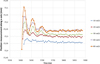Fig. 1 Vibrations of the end effector due to velocity.

Fig. 2 Schematic representation of a flexible joint robot [7].

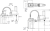Fig. 3 Adept Scara Cobra S600 robot dimensions.

2 Modelling and identification of geometric and dynamic parameters

2.1 Geometric and dynamic modelling

This section provides a brief description on the modelling of the robot. The robot segments are perfectly considered rigid and joints are considered geometrically ideal. Geometric parameters of the robot are presented in Figure 4. O₁ and O₂ are centers of joint 1 and joint 2, G₁ and G₂ are centers of mass of solid 1 and solid 2, q₁ and q₂ are articular values of joint 1 and joint 2, L₁ and L₂ are the length of arm 1 and arm 2, and Lc₁ and Lc₂ are the distance between arm center of mass and joint center of arm 1 and arm 2.

The direct geometric model of the Scara robot is written as:$$\{\begin{array}{c}\hfill x=L_1\cos \left(q_1\right)+L_2\cos \left(q_1+q_2\right)\hfill \\ \hfill y=L_1\sin \left(q_1\right)+L_2\sin \left(q_1+q_2\right)\hfill \end{array}$$(1)where x and y are the coordinates of a point on the end effector in the robot's reference frame $\Re \left(O_1,{\displaystyle \overrightarrow{x}},{\displaystyle \overrightarrow{y}}\right)$.

The inverse dynamic model of the rigid robot is determined using Lagrange method.

This model is linear with respect to dynamic parameters [28]:$${\Gamma }_{\mathbf{m}\mathbf{i}\mathbf{d}}=\mathbf{A}\left(\mathbf{q}\right){\displaystyle \stackrel{\mathrm{}}{\mathbf{q}}}+\mathbf{C}\left(\mathbf{q},{\displaystyle \stackrel{}{\mathbf{q}}}\right){\displaystyle \stackrel{}{\mathbf{q}}}+{\mathbf{F}}_{\mathbf{v}}{\displaystyle \stackrel{}{\mathbf{q}}}+{\mathbf{F}}_{\mathbf{S}}\mathrm{s}\mathrm{i}\mathrm{g}\mathrm{n}\left({\displaystyle \stackrel{}{\mathbf{q}}}\right)$$(2)where ${\Gamma }_{\mathbf{m}\mathbf{i}\mathbf{d}},\mathbf{q},{\displaystyle \stackrel{}{\mathbf{q}}},{\displaystyle \stackrel{\mathrm{}}{\mathbf{q}}}$ respectively represent vectors of motor torques, positions, speeds and joint accelerations. A(q) and $\mathbf{C}\left(\mathbf{q},{\displaystyle \stackrel{}{\mathbf{q}}}\right)$ are two square matrices, the inertia matrix and the Coriolis matrix. F_s and F_v are vectors containing dry and viscous friction coefficients of both joints.

For this case study, we obtain the following model: $$\begin{array}{l}{\Gamma }_{m1}=\left(m_1{L}_{c1}^2+m_2{L}_{c2}^2+m_2{L}_1^2+2L_1{m}_2{L}_{c1}\cos q_2+I_1+I_2\right){{\displaystyle \stackrel{\mathrm{}}{q}}}_1\hfill \\ +\left(m_2{L}_{c2}^2+m_2{L}_1{L}_{c1}\cos q_2+I_2\right){{\displaystyle \stackrel{\mathrm{}}{q}}}_2-2m_2{L}_{c1}{L}_1\sin q_2{{\displaystyle \stackrel{}{q}}}_1{{\displaystyle \stackrel{}{q}}}_2\hfill \\ -m_2{L}_{c1}{L}_1\sin q_2{{\displaystyle \stackrel{}{q}}}_2^2+F_{s1}+F_{v1}{{\displaystyle \stackrel{}{q}}}_1.\hfill \end{array}$$ $$\begin{array}{l}{\Gamma }_{m2}=\left(m_2{L}_{c2}^2+L_1{m}_2{L}_{c1}\cos q_2+I_2\right){{\displaystyle \stackrel{\mathrm{}}{q}}}_1+\left(m_2{L}_{c2}^2+I_2\right){{\displaystyle \stackrel{\mathrm{}}{q}}}_2\hfill \\ +m_2{L}_{c1}{L}_1\sin q_2{{\displaystyle \stackrel{}{q}}}_1^2+F_{s2}+F_{v2}{{\displaystyle \stackrel{}{q}}}_2\hfill \end{array}$$

where m₁ and m₂ are the respective masses of links 1 and 2. I₁ and I₂ are the inertia of solids 1 and 2 along the z-axis at their centre of mass G₁ and G₂.

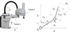Fig. 4 Geometric modeling of the Adept Scara S600 robot.

2.2 Dynamic modelling with flexible articulation of the Scara S600 robot

The robot is modelled as a combination of rigid solid set in motion between them by motorized joints whose transmission system is represented by a spring with a stiffness k_i and a damping coefficient c_i. We note q_i the instruction sent to the articulation motor and q_ei the movement transmitted to the solid after the flexible motion transmission system (Fig. 5).

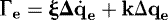
The equations of motion in matrix form are written as: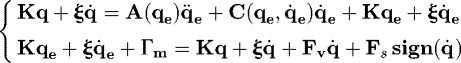$$\{\begin{array}{l}\mathbf{K}\mathbf{q}+\mathbf{\xi }{\displaystyle \stackrel{}{\mathbf{q}}}=\mathbf{A}\left({\mathbf{q}}_{\mathbf{e}}\right){{\displaystyle \stackrel{\mathrm{}}{\mathbf{q}}}}_{\mathbf{e}}+\mathbf{C}\left({\mathbf{q}}_{\mathbf{e}},{{\displaystyle \stackrel{}{\mathbf{q}}}}_{\mathbf{e}}\right){{\displaystyle \stackrel{}{\mathbf{q}}}}_{\mathbf{e}}+\mathbf{K}{\mathbf{q}}_{\mathbf{e}}+\mathbf{\xi }{{\displaystyle \stackrel{}{\mathbf{q}}}}_{\mathbf{e}}\hfill \\ \mathbf{K}{\mathbf{q}}_{\mathbf{e}}+\mathbf{\xi }{{\displaystyle \stackrel{}{\mathbf{q}}}}_{\mathbf{e}}+{\Gamma }_{\mathbf{m}}=\mathbf{K}\mathbf{q}+\mathbf{\xi }{\displaystyle \stackrel{}{\mathbf{q}}}+{\mathbf{F}}_{\mathbf{v}}{\displaystyle \stackrel{}{\mathbf{q}}}+{\mathbf{F}}_s\mathbf{s}\mathbf{i}\mathbf{g}\mathbf{n}({\displaystyle \stackrel{}{\mathbf{q}}})\hfill \end{array}$$(3)where ξ and K are respectively damping and stiffness matrices such that:$$b=\left[\begin{array}{ll}{\xi }_1\hfill & 0\hfill \\ 0\hfill & {\xi }_2\hfill \end{array}\right],\mathbf{K}=\left[\begin{array}{ll}{\kappa }_1\hfill & 0\hfill \\ 0\hfill & {\kappa }_2\hfill \end{array}\right]$$

The system's natural frequencies ω_i and mode quation:$$\left(\left[\mathbf{K}\right]-\left[\mathbf{A}\right]\cdot {\omega }_i^2\right)\cdot \mathbf{Q}=\left(\mathbf{0}\right)$$(4) $$\iff \left[\begin{array}{ll}{k}_1-A_{11}\cdot {\omega }_i^2\hfill & -A_{12}\cdot {\omega }_i^2\hfill \\ -A_{21}\cdot {\omega }_i^2\hfill & k_2-A_{22}\cdot {\omega }_i^2\hfill \end{array}\right]\left\{\begin{array}{c}\hfill q_1\hfill \\ \hfill q_2\hfill \end{array}\right\}=\left\{\begin{array}{c}\hfill 0\hfill \\ \hfill 0\hfill \end{array}\right\}$$

The accuracy of these models is obtained from a modal identification procedure. In a first time, a geometric identification is realized before the identification of dynamic parameters.

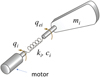Fig. 5 Parameter setting of the dynamic model with flexible joint.

2.3 Geometric identification

The geometric parameters of the model are arm lengths L₁ and L₂. Measurement of the end effector position is carried out using a Leica AT901 Laser Tracker, the target being positioned at the end of the robot at axis 4. According to the Scara geometrical behaviour, we choose to perform the identification using points measured statically during two types of displacements:

• Displacement of q₁ with fixed q₂ (Fig. 6a). The end effector follows a circular trajectory of center O₁. 20 positions are measured over an angle near 45°. A least squares plane P of all these measuring points is then determined as the displacement plane of the end effector. The measured points are then projected into this plane before calculating the least squares circle of these points. We thus determine the position of its center point O₁ in the measuring frame and its radius R.

• Displacement of q₂ with fixed q₁ (Fig. 6b). Trajectory followed by the end-effector is a circle of center O₂ and radius L₂. 14 positions are measured over an angle near 40°. By projecting these points into the plane P and calculating the associated least square circle, we determine the length L₂ and coordinates of O₂ in the measurement frame.

Finally, the length L₁ is determined as the distance between O₁ and O₂. The values identified are: L₁ = 324.489 mm and L₁= 275.019 mm (nominal values are 325 mm for L₁ and 275 mm for L₂). These results are validated on 5 randomly selected positions in the workspace. For these 5 positions, mean error between calculated positions by the direct geometric model and those measured by the laser is 0.2 mm and the standard deviation is 0.03 mm.

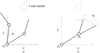Fig. 6 Displacements made during the identification of geometric parameters. (a) Movement of q2 with q2 fixed. (b) Movement of q2 with q1 fixed.

2.4 Dynamic parameters identification

Dynamic parameters are different kind of quantity (stiffness, damping, inertia, friction and position of mass centre). These parameters have to be identified with different type of data.

2.4.1 Identification of joint stiffness and damping

The identification of the joint stiffness and damping can be done from the determination of system's natural frequencies by modal analysis (Fig. 7). The modal analysis is performed using LMS-TAB software.

Three configurations have been chosen to measure natural frequencies of the robot: extended arm (q₂ = 0°), arm bent at 45° (q₂= 45°) and arm bent at 90° (q₂ = 90°). Once the accelerometers are in place, the measurement protocol is done in two steps:

Step 1: we apply an excitation force at the end effector using an impact hammer.

Step 2: After choosing the bandwidth for signal acquisition, the frequencies are then selected manually by using PolyMax identification procedure. The software proposes unstable and stable modes representative of numerical or structural modes for the results. Then, only the so-called “stable” modes are selected.

Observation of the modal shape of the model shows that the first 2 modes are associated to the deformation of joints 1 and 2.

For the identification of stiffness and damping parameters of joints 1 and 2, the first 2 modes are considered (Tab. 1).

The others dynamic parameters are then identified from motor torque measurement.

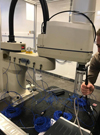Fig. 7 Experimental setup of modal analysis.

2.4.2 Dynamic identification

According to equations (2), (10) parameters must be identified for the rigid dynamic model:$$\left(m_1{m}_2{L}_{c1}{L}_{c2}{I}_1{I}_2{F}_{s1}{F}_{s2}{F}_{v1}{F}_{v2}\right).$$

The identification procedure is done in four steps using the same trajectory performed at different speeds:

Step 1: The robot goes from position A to position B in the joint space.

Step 2: The torque is not directly measurable. It is deduced from the measurement of the motor current by the following relationship for axis j:$${\Gamma }_{me{s}_j}=v_j\ast K_j,K_j=R_j\ast g_j\ast K_T$$(5)where v_j is the value of the motor current, R_j the reduction ratio of the joint, g_j the static gain of the amplifier, K_T the torque coefficient of the motor.

Step 3: We calculate the torque Γ_mdi from equation (2). To do so, we measure the angular position with the encoder of each motorized axis. The estimation of acceleration and speed is then computed by numerical derivation and Butterworth filtering of this last measurement [29,30].

Step 4: The identification procedure is achieved by minimizing the following cost function:$$f_{co{\displaystyle \stackrel{}{u}}t}={\sum }_i{\left({\Gamma }_{mes}\left(t\right)-{\Gamma }_{mdi}\left(t\right)\right)}^2$$(6)

First of all, the dry friction parameters were identified using a low speed movement (axis by axis). The trajectory is composed of two movements: firstly, movement of q₁ with fixed q₂ and secondly, movement of q₂ with fixed q₁ (Fig. 8).

For the rest of the parameters, trajectory is the same as before but with higher speed. Measured torques during movement of axis 1 and then axis 2 are isolated and used to perform the identification. After optimization (Fig. 9), the mean error is 0.648 N m and the standard deviation is 1.676 N m.

To identify the stiffness of the joints, we couple the cost function expressed by equation (6) with another cost function which compares the natural frequencies measured with the modal analysis and estimated by the model (Eq. (4)). Values of these modes varies according to q₂ as the inertia matrix is a function of q₂ (Eq. (2)). Identified parameters are found in Table 2. The parameters already identified in the previous section are validated with a random trajectory made by the end effector. The mean error is 1.4 N.m and standard deviation is 3 N m.

To finalize the identification process, damping parameters values have to be determined.

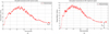Fig. 8 Dry friction identification. (a) Dry friction joint 1. (b) Dry friction joint 2.

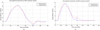Fig. 9 Measured and calculated torque. (a) Motor 1: Measured and calculated torque. (b) Motor 2: Measured and calculated torque.

2.4.3 Damping identification

The modal analysis allowed us to determine the two modes corresponding to deformations of joint 1 and joint 2. Damping ratios are evaluated for these two modes. We only consider the first extended arm configuration for identifying joint damping because all accelerometers and hammer chock are oriented tangent to the displacement of joint 1 and 2. Thus, in this configuration, joints are directly loaded by hammer chock and their vibration amplitudes are directly measured by accelerometers. This makes it possible to link the measured damping to the torsional damping at each joint. Finally, damping coefficients of joint 1 and joint 2 are deduced from measured damping ratios (ζ) for these two modes according to robot configuration using the following relation:$${\mathbf{C}}_{\mathbf{d}}=2\cdot \varsigma \cdot \sqrt{{\mathbf{K}}_{\mathbf{d}}{\mathbf{A}}_{\mathbf{d}}}$$where ς is the measured damping ratio matrix and C_d, K_d, A_d respectively the diagonalized matrixes of joint damping, stiffness and inertia. Damping parameters are finally determined as follows, c₁=57.484 N.m.s. rad⁻¹ and c₂= 12.983 N.m.s. rad⁻¹.

After the identification process, the identified model is used to define a model-based control law.

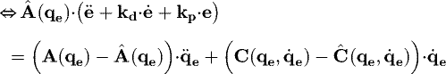
3 Model based flexible control (MBC) law

In this chapter we develop a computed torque control law taking into consideration joint flexibilities. Validity and benefit of this control law for flexible joint robot is evaluated through advanced simulations. All the values of identified parameters in previous chapter is integrated in the simulator in order to have a representation as close as possible to the real behaviour of robot. Before reaching this stage, we define a trajectory generator in the articular space, and develop a methodology for tune gains of the used corrector in order to compare similarly different kind of control laws.

3.1 Control law scheme

The equation of motion governing the variable qe is obtained from the relationship (3):$${\Gamma }_{\mathbf{m}}=\mathbf{\xi }\mathbf{\Delta }{{\displaystyle \stackrel{\Delta }{\mathbf{q}}}}_{\mathbf{e}}+\mathbf{k}\mathbf{\Delta }{\mathbf{q}}_{\mathbf{e}}+{\mathbf{F}}_{\mathbf{s}}\cdot \mathbf{s}\mathbf{i}\mathbf{g}\mathbf{n}\left({\displaystyle \stackrel{}{\mathbf{q}}}\right)+{\mathbf{F}}_{\mathbf{v}}\cdot {\displaystyle \stackrel{}{\mathbf{q}}}$$(7) $${\Gamma }_{\mathbf{e}}=\mathbf{\xi }\mathbf{b}{{\displaystyle \stackrel{}{\mathbf{q}}}}_{\mathbf{e}}+\mathbf{k}\Delta {\mathbf{q}}_{\mathbf{e}}$$ $${\Gamma }_{\mathbf{e}}={\Gamma }_{\mathbf{m}}-{\mathbf{F}}_{\mathbf{s}}\cdot \mathbf{s}\mathbf{i}\mathbf{g}\mathbf{n}\left({\displaystyle \stackrel{}{\mathbf{q}}}\right)-{\mathbf{F}}_{\mathbf{v}}\cdot {\displaystyle \stackrel{}{\mathbf{q}}}$$ $$\leftrightarrow \mathbf{b}{\mathbf{q}}_{\mathbf{e}}=\frac{{\Gamma }_{\mathbf{e}}}{\mathbf{k}+\mathbf{p}\cdot \mathbf{\xi }}=\frac{{\Gamma }_{\mathbf{m}}-F_{\mathbf{s}}\cdot \mathbf{s}\mathbf{i}\mathbf{g}\mathbf{n}\left({\displaystyle \stackrel{}{\mathbf{q}}}\right)-{\mathbf{F}}_{\mathbf{v}}\cdot {\displaystyle \stackrel{}{\mathbf{q}}}}{\mathbf{k}+\mathbf{p}\cdot \mathbf{\xi }}(\text{Laplace}\text{transform})$$where Γ_m and Γ_e are respectively the motor torque and the elastic torque, and Δq_e = q − q_e.

On the other hand, the equation of motion is written as:$${\Gamma }_{\mathbf{m}}=\mathbf{A}\left({\mathbf{q}}_{\mathbf{e}}\right)\cdot {{\displaystyle \stackrel{\mathrm{}}{\mathbf{q}}}}_{\mathbf{e}}+\mathbf{C}\left({\mathbf{q}}_{\mathbf{e}},{{\displaystyle \stackrel{}{\mathbf{q}}}}_{\mathbf{e}}\right)\cdot {{\displaystyle \stackrel{}{\mathbf{q}}}}_{\mathbf{e}}+{\mathbf{F}}_{\mathbf{v}}\cdot {\displaystyle \stackrel{}{}}{}_{}{\displaystyle \stackrel{}{\mathbf{q}}}+{\mathbf{F}}_{\mathbf{s}}\cdot \mathbf{s}\mathbf{i}\mathbf{g}\mathbf{n}\left({\displaystyle \stackrel{}{\mathbf{q}}}\right)$$(8)where q_e = q − Δq_e.

These two relationships (Eqs. (7) and (8)) are the basis of the new control law based on the dynamic model of a manipulator with flexible joints. Flexibility of joints is presented in the control diagram as a feedback loop (orange block). In absence of gravity effect, PD control strategies are asymptotically stable and do not require addition of an integrator [31]. The control scheme corresponding to this computed torque control law is defined in Figure 10.

To validate and to illustrate the benefit and limit of the proposed control law, firstly, we develop an advanced simulation with Adams' and Simulink. Secondly, we make a comparative analysis with two control strategies applied to same simulator. Simulations results are presented in a comparative table.

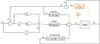Fig. 10 New computed torque control law for flexible joint manipulator (MBC).

3.2 Adams simulink co-simulation unit

The numeric model of a robot with 2 degrees of freedom was developed in Adams software. The idea is to use its mechanism solver to simulate robot motion generated by discretised setpoint computed by the control law. The dimensions and dynamic characteristics correspond to the one identified on the Scara S600 robot of SIGMA Clermont's technological platform. The control laws are implemented in Simulink. The numeric model defined in Adams is set in motion via a co-simulation. The flexibility of the connections is represented under Adams by a linear torsion spring modelled by stiffness and damping. Two segments of negligible mass compared to that of the two robot axes (m₁ = m₂ = 0.15 kg) are added to perform the simulation with flexible connections. The movement of these two segments is controlled. The segments are in rotational connection with the robot elements and the movement is transmitted by the springs. The robot model is defined geometrically and dynamically using the parameters identified above.

3.3 Trajectory generation and gain correction

To be consistent with a classical robotized path, the trajectory followed in this work is described with a five-degree polynomial function, which ensures a position, velocity and acceleration movement continuities without excessive dynamic load (Fig. 11). The maximum velocity and acceleration are those of Scara robot (max velocity: joint 1: 386 deg/s and joint 2: 720 deg/s; max acceleration: joint 1: 386 deg/s² and joint 2: 720 deg/s²).

Gain tuning is realized to avoid oscillations, and in accordance with the response time at 5% (t_r 5%) of position loop. Thus, an appropriate adjustment [20] is: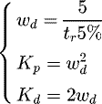$$\{\begin{array}{l}{w}_d=\frac{5}{t_{r}5\%}\hfill \\ K_p=w_d^2\hfill \\ K_d=2w_d\hfill \end{array}$$(9)where K_p and K_d represents respectively proportional and derivative gains of the PD corrector. In the following paragraph, we develop a robot position control using the co-simulation tool Adams and Simulink. Initially, the robot is positioned in a configuration where arms are perpendicular. Initial and desired operational and Cartesian positions of the robot end effector are defined in Table 3.

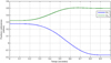Fig. 11 Program tool path in the cartesian space.

3.3.1 Modal based control (MBC) law

This control law is our new computed torque control law for flexible joint manipulator.

The gain setting used is the one defined in equation (9). For this law, we choose a response time at 5%(t_r 5%) of 0.0143 seconds for an adequate setting. Thus 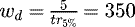$w_d=\frac{5}{t{r}_{5\%}}=350$, the gains obtained for the two rotation axes are K_d1 = K_d2 = 700 and Kp₁ = Kp₂ = 122500. Evolution curves of the positioning error in both joint and Cartesian spaces are shown in Figure 12a.

Desired position is reached with a maximum trajectory tracking error of 1 millimetre along x-direction and half a millimetre in y-direction. The mean errors and standard deviation are in the order of 10⁻⁴ meters and 10⁻⁶ radians in Cartesian and articular spaces, respectively. At the end of the task, robot's behaviour is stable, positioning error is 10⁻⁹ meters and an accuracy of 1 µm is achieved after 0.913 s.

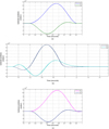Fig. 12 Joint and Cartesian positioning errors. (a) Cartesian positionning errors for MBC. (b) Cartesian positionning errors for rigid control. (c) Cartesian positionning errors for feedforward control.

3.3.2 Rigid control

In order to show the benefit to consider flexibilities in the control loop, a control law dedicated to rigid robots (Fig. 13) is applied to the same Adams robot model with flexible joints.

The gain tuning used to minimize the error is defined in the equation (9). For a t_r 5% of 0.0143 seconds (identical to that of the MBC control law), joint flexibilities are highly stressed, vibrations appear, and desired positions are never reached because the robot never converges to a fixed position. The system stabilizes for a t_r 5% of 0.3846 seconds, and the proportional and derivative gains are 169 and 26, respectively.

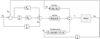Fig. 13 Control law dedicated to rigid robots applied to robots with joint flexibility.

3.3.3 Feedforward control

In this section, a feedforward control combined with a PD control is applied to the same simulator (Fig. 14). An adequate adjustment [19] of the K_p and K_d gains to control the transient behaviour of the error is:$$\{\begin{array}{c}\hfill {\mathit{K}}_{\mathit{p}}={\mathit{a}}_{{11}}{\mathit{w}}_{\mathit{d}}^{\mathit{2}}\hfill \\ \hfill {\mathit{K}}_{\mathit{d}}={2}{\mathit{a}}_{{11}}\mathit{\xi }{\mathit{w}}_{\mathit{d}}-{\mathit{c}}_{{11}}\hfill \end{array}\text{and}\{\begin{array}{c}\hfill {\mathit{w}}_{\mathit{d}}=\frac{{5}}{{\mathit{t}}_{\mathit{r}}{5}{\%}}\hfill \\ \hfill \mathit{\xi }={1}\hfill \end{array}$$(10) where the element a₁₁ designate maximum value of matrix A_max and has the value 1.9117. Similarly, c₁₁ has the value 1.14. For a proper gain adjustment, t_r 5% is fixed at 0.103 seconds. Thus, the gains obtained for both rotational axes are: Kp = 182 and K_d = 4441.

Results of the simulations are presented in Figure 12 and in the comparative balance sheet table (Tab. 4).

As a quick interpretation, MBC control law (considering joint flexibilities as a feedback loop in the control diagram) provides an additional performance advantage over all other control laws in terms of end effector placement accuracy and stability time with a benefit of 10% and 50% according to feedforward and rigid control respectively (Pick and Place operation requirements).

However, model-based control law can be sensitive to identification errors. A sensitivity analysis ensures to determine critical parameters for such control law strategy.

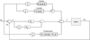Fig. 14 Feedforward control.

4 Sensitivity analysis

This sensitivity analysis ensures to determine critical flexible joint parameters with regard to vibration decreasing. The fact that we use a model-based control law strategy allows us to only focus on the influence of mechanical parameters used to describe joint behaviour.

The torques applied to flexible connections, according to estimated dynamic parameters ${\displaystyle \hat{\mathbf{\chi }}}$, are obtained from the following model:$${\Gamma }_{\mathbf{m}}={\displaystyle \hat{\mathbf{A}}}\left({\mathbf{q}}_{\mathbf{e}}\right)\cdot \mathbf{U}+{\displaystyle \hat{\mathbf{C}}}\left({\mathbf{q}}_{\mathbf{e}},{{\displaystyle \stackrel{}{\mathbf{q}}}}_{\mathbf{e}}\right)\cdot {{\displaystyle \stackrel{}{\mathbf{q}}}}_{\mathbf{e}}+{{\displaystyle \hat{\mathbf{F}}}}_{\mathbf{s}}\cdot \mathrm{s}\mathrm{i}\mathrm{g}\mathrm{n}\left({\displaystyle \stackrel{}{\mathbf{q}}}\right)+{{\displaystyle \hat{\mathbf{F}}}}_{\mathbf{v}}\cdot {\displaystyle \stackrel{}{\mathbf{q}}}$$(11)where ${\displaystyle \hat{\mathbf{A}}}={\mathbf{A}}_{\left({\displaystyle \hat{\mathbf{x}}}\right)}\text{et}{\displaystyle \hat{C}}={\mathbf{C}}_{\left({\displaystyle \hat{u}}\right)}$ 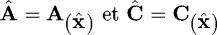and ∧ is the symbol of estimation notion.

Thus, control law U is defined by the following relationship:$$\mathbf{U}={{\displaystyle \stackrel{\mathrm{}}{\mathbf{q}}}}_{\mathbf{d}}+{\mathbf{k}}_{\mathbf{p}}\cdot \mathbf{e}+{\mathbf{k}}_{\mathbf{d}}\cdot {\displaystyle \stackrel{}{\mathbf{e}}}$$(12)where $\mathbf{e}={\mathbf{q}}_{\mathbf{d}}-{\mathbf{q}}_{\mathbf{e}},{\displaystyle \stackrel{}{\mathbf{e}}}={{\displaystyle \stackrel{}{\mathbf{q}}}}_{\mathbf{d}}-{{\displaystyle \stackrel{}{\mathbf{q}}}}_{\mathbf{e}},{\displaystyle \stackrel{\mathrm{}}{\mathbf{e}}}={{\displaystyle \stackrel{\mathrm{}}{\mathbf{q}}}}_{\mathbf{d}}-{{\displaystyle \stackrel{\mathrm{}}{\mathbf{q}}}}_{\mathbf{e}}$

Let consider that equation (3) is equal to equation (11):$$\begin{array}{l}{\displaystyle \hat{\mathbf{A}}}\left({\mathbf{q}}_{\mathbf{e}}\right)\cdot \mathbf{U}+{\displaystyle \hat{\mathbf{C}}}\left({\mathbf{q}}_{\mathbf{e}},{{\displaystyle \stackrel{}{\mathbf{q}}}}_{\mathbf{e}}\right)\cdot {{\displaystyle \stackrel{}{\mathbf{q}}}}_{\mathbf{e}}+{{\displaystyle \hat{\mathbf{F}}}}_{\mathbf{s}}\cdot \mathrm{s}\mathrm{i}\mathrm{g}\mathrm{n}\left({\displaystyle \stackrel{}{\mathbf{q}}}\right)+{{\displaystyle \hat{\mathbf{F}}}}_{\mathbf{v}}\cdot {\displaystyle \stackrel{}{\mathbf{q}}}=\mathbf{A}\left({\mathbf{q}}_{\mathbf{e}}\right)\cdot {{\displaystyle \stackrel{\mathrm{}}{\mathbf{q}}}}_{\mathbf{e}}+\mathbf{C}\left({\mathbf{q}}_{\mathbf{e}},{{\displaystyle \stackrel{}{\mathbf{q}}}}_{\mathbf{e}}\right)\cdot {{\displaystyle \stackrel{}{\mathbf{q}}}}_{\mathbf{e}}+\hfill \\ {\mathbf{F}}_{\mathbf{s}}\cdot \mathrm{s}\mathrm{i}\mathrm{g}\mathrm{n}\left({{\displaystyle \stackrel{}{\mathbf{q}}}}_{\mathbf{e}}\right)+{\mathbf{F}}_{\mathbf{v}}\cdot {{\displaystyle \stackrel{}{\mathbf{q}}}}_{\mathbf{e}}\hfill \end{array}$$(13)

By substituting U with its expression in equation (12) and eliminating the terms of dry and viscous friction on both sides of this equality, equation (13) becomes:$${\displaystyle \hat{\mathbf{A}}}\left({\mathbf{q}}_{\mathbf{e}}\right)\cdot \left({{\displaystyle \stackrel{\mathrm{}}{\mathbf{q}}}}_{\mathbf{d}}+{\mathbf{k}}_{\mathbf{p}}\cdot \mathbf{e}+{\mathbf{k}}_{\mathbf{d}}\cdot {\displaystyle \stackrel{}{\mathbf{e}}}\right)+{\displaystyle \hat{\mathbf{C}}}\left({\mathbf{q}}_{\mathbf{e}},{{\displaystyle \stackrel{}{\mathbf{q}}}}_{\mathbf{e}}\right)\cdot {{\displaystyle \stackrel{}{\mathbf{q}}}}_{\mathbf{e}}=\mathbf{A}\left({\mathbf{q}}_{\mathbf{e}}\right)\cdot {{\displaystyle \stackrel{\mathrm{}}{\mathbf{q}}}}_{\mathbf{e}}+\mathbf{C}\left({\mathbf{q}}_{\mathbf{e}},{{\displaystyle \stackrel{}{\mathbf{q}}}}_{\mathbf{e}}\right)\cdot {{\displaystyle \stackrel{}{\mathbf{q}}}}_{\mathbf{e}}$$

By adding and subtracting ${\displaystyle \hat{\mathbf{A}}}\left({\mathbf{q}}_{\mathbf{e}}\right)\cdot {{\displaystyle \stackrel{\mathrm{}}{\mathbf{q}}}}_{\mathbf{e}}$ we obtain:$$\iff {\displaystyle \hat{\mathbf{A}}}\left({\mathbf{q}}_{\mathbf{e}}\right)\cdot \left({\mathbf{k}}_{\mathbf{p}}\cdot \mathbf{e}+{\mathbf{k}}_{\mathbf{d}}\cdot {\displaystyle \stackrel{}{\mathbf{e}}}\right)=\mathbf{A}\left({\mathbf{q}}_{\mathbf{e}}\right)\cdot {{\displaystyle \stackrel{\mathrm{}}{\mathbf{q}}}}_{\mathbf{e}}-{\displaystyle \hat{\mathbf{A}}}\left({\mathbf{q}}_{\mathbf{e}}\right)\cdot {{\displaystyle \stackrel{\mathrm{}}{\mathbf{q}}}}_{\mathbf{d}}+\mathbf{C}\left({\mathbf{q}}_{\mathbf{e}},{{\displaystyle \stackrel{}{\mathbf{q}}}}_{\mathbf{e}}\right)\cdot {{\displaystyle \stackrel{}{\mathbf{q}}}}_{\mathbf{e}}-{\displaystyle \hat{\mathbf{C}}}\left({\mathbf{q}}_{\mathbf{e}},{{\displaystyle \stackrel{}{\mathbf{q}}}}_{\mathbf{e}}\right)\cdot {{\displaystyle \stackrel{}{\mathbf{q}}}}_{\mathbf{e}}+{\displaystyle \hat{\mathbf{A}}}\left({\mathbf{q}}_{\mathbf{e}}\right)\cdot {{\displaystyle \stackrel{\mathrm{}}{\mathbf{q}}}}_{\mathbf{e}}-{\displaystyle \hat{\mathbf{A}}}\left({\mathbf{q}}_{\mathbf{e}}\right)\cdot {{\displaystyle \stackrel{\mathrm{}}{\mathbf{q}}}}_{\mathbf{e}}$$ $$\iff {\displaystyle \hat{\mathbf{A}}}\left({\mathbf{q}}_{\mathbf{e}}\right)\cdot \left({\displaystyle \stackrel{\mathrm{}}{\mathbf{e}}}+{\mathbf{k}}_{\mathbf{d}}\cdot {\displaystyle \stackrel{}{\mathbf{e}}}+{\mathbf{k}}_{\mathbf{p}}\cdot \mathbf{e}\right)=\left(\mathbf{A}\left({\mathbf{q}}_{\mathbf{e}}\right)-{\displaystyle \hat{\mathbf{A}}}\left({\mathbf{q}}_{\mathbf{e}}\right)\right)\cdot {{\displaystyle \stackrel{\mathrm{}}{\mathbf{q}}}}_{\mathbf{e}}+\left(\mathbf{C}\left({\mathbf{q}}_{\mathbf{e}},{{\displaystyle \stackrel{}{\mathbf{q}}}}_{\mathbf{e}}\right)-{\displaystyle \hat{\mathbf{C}}}\left({\mathbf{q}}_{\mathbf{e}},{{\displaystyle \stackrel{}{\mathbf{q}}}}_{\mathbf{e}}\right)\right)\cdot {{\displaystyle \stackrel{}{\mathbf{q}}}}_{\mathbf{e}}$$(14)

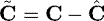Let: ${\displaystyle \tilde{\mathbf{A}}}=\mathbf{A}-{\displaystyle \hat{\mathbf{A}}}$ and ${\displaystyle \tilde{\mathbf{C}}}=\mathbf{C}-{\displaystyle \hat{\mathbf{C}}}$ equation (14) can finally be written as follows:$${\displaystyle \stackrel{\mathrm{}}{\mathbf{e}}}+{\mathbf{k}}_{\mathbf{d}}\cdot {\displaystyle \stackrel{}{\mathbf{e}}}+{\mathbf{k}}_p\cdot \mathbf{e}={\displaystyle \hat{\mathbf{A}}}{\left({\mathbf{q}}_{\mathbf{e}}\right)}^{-1}\left({\displaystyle \tilde{\mathbf{A}}}\left({\mathbf{q}}_{\mathbf{e}}\right)\cdot {{\displaystyle \stackrel{\mathrm{}}{\mathbf{q}}}}_{\mathbf{e}}+{\displaystyle \tilde{\mathbf{C}}}\left({\mathbf{q}}_{\mathbf{e}},{{\displaystyle \stackrel{}{\mathbf{q}}}}_{\mathbf{e}}\right)\cdot {{\displaystyle \stackrel{}{\mathbf{q}}}}_{\mathbf{e}}\right)$$(15)

Normally, the error and its derivative converge towards 0 in a second order determined by the servo gains. However, in equation (15), the second member is not null but depends on identify values of inertial parameters and joint flexibilities (stiffness and damping). Hence, this equation illustrates the need to take into consideration the joint flexibility in the control. These three parameters are subject to estimation inaccuracies. A sensitivity study is conduced to quantify the impact of these errors on the vibration behaviour. This sensitivity analysis is realised by isolating each source of error in order to determine its influence separately by numerical simulations.

4.1 Errors in the estimation of inertia

In order to study the influence of inertial values on the performance of our new model-based control (MBC) law, we realise several simulations of the MBC control law (with same settings of PD gains) with 2% error steps on inertial parameters. For errors below 12%, simulation results confirm that the control is able to adapt avoid vibrations at the end of the movement. Starting from 12%, vibrations related to instability phenomena appear.

4.2 Errors in joint stiffness

The relevance of MBC is evaluated for a case where values of joint stiffness present defect with regard to implemented one in Adams model. In this purpose, we apply the same test as before but with a 1% error step (since the impact of these errors is then greater). Simulations reveals that vibrations appears from errors of 3% in joint stiffness. These vibrations can be controlled by minimizing the performance of the control law due to an increase in response time at 5% (t_r 5%) and consequently a decrease in the corrector gains.

4.3 Errors in joint damping

The impact of these errors is significantly very important. Vibrations appear from a 3% error on damping. These vibrations can be controlled by minimizing the performance of the control law due to an increase in response time at 5% (t_r 5%) and consequently a decrease in the corrector gains.

Table 5 resume all the sensitivity test and the decreasing of performances due to an increasing of t_r 5%. Thus, we can show that damping and stiffness is critical parameters for vibration control. However, there is work on stiffness joint robot identification and just few on damping. Thus, this work demonstrates a huge need to develop accurate methodology to identify joint damping parameter.

5 Conclusion

In this work we have developed a new model-based control law dedicated to manipulators with flexible joints to control vibrations behaviour during Pick and Place operations. Simulations are applied on a Scara robot with 2 Degree of freedom, so that this law is applicable to more complex structures. We have modelled and identified the geometric and dynamic parameters of a Sacra robot including friction, stiffness and damping. MBC law dedicated to robots with joints flexibility is then developed using Simulink after defining the trajectory and PD correction system. Advanced simulations results in terms of response time and maximum and average trajectory errors clearly shows the relevance of the proposed approach integrating joint flexibilities as a feedback loop in control diagram. In parallel, its performance is validated due to comparisons with other control laws. Finally, we concluded this work by a sensitivity analysis to modelling errors. We demonstrate, by calculations, that joint flexibilities and damping are influential on the modelling error which indicates the importance of taking them into consideration for the control accuracy of robot vibrations.

Nomenclature

A(q): The inertia matrix

$\mathbf{\text{C}}\left(\mathbf{\text{q,q}}\right)$ : Coriolis matrix

ξ : Damping matrix

F_s : Vector containing dry friction coefficients of joints

F_v : Vector containing viscous friction coefficients of joints

O_i : Center of joint i

G_i : Center of mass of solid i

g_j : Static gain of the amplifier

Γ_mdi : Vectors of motor torques

Γ_m : Motor torque

Γ_e : Elastic torque

I_i : Inertia of solids i along the z-axis

K : Stiffness matrix

K_p and K_d : Respectively proportional and derivative gains of the PD corrector

K_T : Torque coefficient of the motor

L_i : ith arm length

L_ci : Distance between ith arm center of mass G_i and ith joint center Oi

m_i : Masses of links i

v_j : Motor current

ω_i : System's natural frequencies

$\text{q,q,q}$ : Positions, speeds and joint accelerations

q_ei : The movement transmitted to the solid after the flexible motion transmission system

q_i : Instruction sent to the motor

$\Re \left(O_1,{\displaystyle \overrightarrow{x}},{\displaystyle \overrightarrow{y}}\right)$ : Robot's reference frame

Rj : Reduction ratio of the joint

(x,y): Coordinates of a point on the end effector in the robot's reference frame

ς : Measured damping ratio matrix

${\displaystyle \hat{\chi }}$ : Estimated dynamic parameters

Acknowledgments

This work was supported by a PhD funding from the city of AL ABDEH (LIBAN).

References

All Tables

All Figures

	Fig. 1 Vibrations of the end effector due to velocity.
In the text

	Fig. 2 Schematic representation of a flexible joint robot [7].
In the text

	Fig. 3 Adept Scara Cobra S600 robot dimensions.
In the text

	Fig. 4 Geometric modeling of the Adept Scara S600 robot.
In the text

	Fig. 5 Parameter setting of the dynamic model with flexible joint.
In the text

	Fig. 6 Displacements made during the identification of geometric parameters. (a) Movement of q2 with q2 fixed. (b) Movement of q2 with q1 fixed.
In the text

	Fig. 7 Experimental setup of modal analysis.
In the text

	Fig. 8 Dry friction identification. (a) Dry friction joint 1. (b) Dry friction joint 2.
In the text

	Fig. 9 Measured and calculated torque. (a) Motor 1: Measured and calculated torque. (b) Motor 2: Measured and calculated torque.
In the text

	Fig. 10 New computed torque control law for flexible joint manipulator (MBC).
In the text

	Fig. 11 Program tool path in the cartesian space.
In the text

	Fig. 12 Joint and Cartesian positioning errors. (a) Cartesian positionning errors for MBC. (b) Cartesian positionning errors for rigid control. (c) Cartesian positionning errors for feedforward control.
In the text

	Fig. 13 Control law dedicated to rigid robots applied to robots with joint flexibility.
In the text

	Fig. 14 Feedforward control.
In the text

References

- ISO 9283, Manipulating Industrial Robots − Performance Criteria and Related Test Methods, 1993 [Google Scholar]
- F. Colas, Synthèse et réglage de lois de commande adaptées aux axes souples en translation − Application aux robots cartésiens 3 axes, Thèse, École Centrale de Lille, 2007 [Google Scholar]
- M. Oueslati, Contribution à la modélisation dynamique, l'identification et la synthèse de lois de commande adaptées aux axes flexibles d'un robot industriel, Thèse, Arts et Métiers ParisTech − Centre de Lille, 2013 [Google Scholar]
- C. Dumas, S. Caro, S. Garnier, Joint stiffness identification of six-revolute industrial serial robots, Robot. Comput. Integr. Manuf. 27 (2011) [Google Scholar]
- K. Melhem, W. Wang, S. Member, Global output tracking control of flexible joint robots via factorization of the manipulator mass matrix, IEEE Trans. Robot. 25, 2 (2009) [Google Scholar]
- G. Xiong, Y. Ding, L. Zhu, Stiffness-based pose optimization of an industrial robot for five-axis milling, Robot. Comput. Integr. Manufactur. 55 (2019) [CrossRef] [Google Scholar]
- S. Mejri, Identification et modélisation du comportement dynamique des robots d'usinage, Thèse, Université Blaise Pascal − Clermont II, 2016 [Google Scholar]
- J. Kima, E.A. Croftb, Preshaping input trajectories of industrial robots for vibration suppression, Robot. Comput. Integr. Manufactur. 54 (2018) [Google Scholar]
- B. Siciliano, O. Khatib, Handbook of Robotics Springer, (2008) [Google Scholar]
- H.N. Rahimi, M. Nazemizadeh, Dynamic analysis and intelligent control techniques for fl exible manipulators: a review, Adv. Robot. 28, 2 (2014) [Google Scholar]
- M. Sayahkarajy, Z. Mohamed, A.A.M. Faudzi, Review of modelling and control of flexible-link manipulators, J. Syst. Control Eng. (2016) [Google Scholar]
- L.M. Sweet, K.L. Strobel, Dynamic models for control system design of integrated robot and drive systems, J. Dyn. Syst. Meas. Control 107 (2015) [Google Scholar]
- M. Makarov, M. Grossard, P. Rodriguez-Ayerbe, D. Dumur, A frequency-domain approach for flexible-joint robot modeling and identification, IFAC Proc. 45, 16 (2012) [Google Scholar]
- F. Ghorbel, J.Y. Hung, M.W. Spong, Adaptive control of flexible joint manipulators, in Proceedings, 1989 International Conference on Robotics and Automation , 1989, no. 2, pp. 1188– 1193 [Google Scholar]
- R.V.P. and A.J.A.-K. RA. AI-Ashoor, K. Khorasani, Adaptive control of flexible joint manipulators, IEEE J. Robot. Autom. (1990) [Google Scholar]
- S. Moberg, Modeling and Control of Flexible Manipulators, Report, Linköping University, 2010 [Google Scholar]
- A.S. Andreev, O.A. Peregudova, A.A. Sobolev, On Global Trajectory Tracking Control of Robot Manipulators with Flexible Joints, IFAC PapersOnLine 51, 32 (2018) [Google Scholar]
- P. Hamon, M. Gautier, P. Garrec, New dry friction model with load- and velocity- dependence and dynamic identification of multi-dof robots, in International Conference on Robotics and Automation , 2015 [Google Scholar]
- A.C. Bittencourt, E. Wernholt, S. Sander-Tavallaey, T. Brogårdh, An extended friction model to capture load and temperature effects in robot joints, in IEEE/RSJ 2010 International Conference on Intelligent Robots and Systems, IROS 2010 − Conference Proceedings , 2010, pp. 6161– 6167 [Google Scholar]
- T. Zou, F. Ni, C. Guo, H. Liu, Parameter Identification and Controller Design for Flexible Joint of Chinese Space Manipulator, in International Conference on Robotics and Biomimetics , 2014, pp. 142– 147 [Google Scholar]
- M.J. Kim, F. Beck, C. Ott, A. Albu-Schaeffer, Model-free friction observers for flexible joint robots with torque measurements, IEEE Trans. Robot. 1−8 (2019) [Google Scholar]
- M. Östring, S. Gunnarsson, M. Norrlöf, Closed-loop identification of an industrial robot containing flexibilities, Control Eng. Pract. 11, 3 (2003) [Google Scholar]
- R. Hopler, M. Thummel, Symbolic computation of the inverse dynamics of elastic joint robots, in IEEE Int. Conf. Robot. Autom. 2004. Proceedings. ICRA '04. 2004 , vol. 5, April, pp. 4314–4319, 2004 [Google Scholar]
- W. Khalil, E. Dombre, Bases de la modélisation et de la commande des robots robots-manipulateurs de type série, 2012, pp. 1–52 [Google Scholar]
- J. Le Flohic, Vers une commande basée modèle des machines complexes: application aux machines-outils et machines d'essais mécaniques, Thèse, Université Blaise Pascal − Clermont II, 2015 [Google Scholar]
- M. Makarov, Contribution à la modélisation et la commande robuste de robots manipulateurs à articulations flexibles. Applications à la robotique interactive, Thèse, Supélec, 2013 [Google Scholar]
- P. Tomei, A simple PD controller for robots with elastic joints − automatic control, IEEE Trans. 36, 10 (1991) [Google Scholar]
- M. Gautier, Contribution à la modélisation et à l'identification des robots, Thèse, Université de Nantes, École Nationale Supérieure de Mécanique, 1990 [Google Scholar]
- O.A. Vivas, Contribution à l'identification et à la commande des robots parallèles, Thèse, Université de Montpellier II, 2005 [Google Scholar]
- Q. Guo, W. Perruquetti, M. Gautier, On-line robot dynamic identification based on power model, modulating functions and causal Jacobi estimator, in IEEE International Conference on Robotics and Automation , 1997, pp. 1922– 1927 [Google Scholar]
- R. Lozano, A. Valera, P. Albertos, S. Arimoto, T. Nakayama, PD control of robot manipulators with joint flexibility, actuators dynamics and friction, Automatica 35, (1999) [Google Scholar]
Cite this article as: J. Farah, H. Chanal, N. Bouton, V. Gagnol, A model-based control law for vibration reduction of serial robots with flexible joints, Mechanics & Industry 22, 38 (2021)