| Issue |
Mechanics & Industry
Volume 27, 2026
Robotic Process Automation for Smarter Devices in Manufacturing
|
|
|---|---|---|
| Article Number | 14 | |
| Number of page(s) | 14 | |
| DOI | https://doi.org/10.1051/meca/2026009 | |
| Published online | 03 April 2026 | |
Original Article
Design of cascaded FOPI-FOPD-BLQG controller tuned with hybrid grasshopper and firefly algorithms for stabilizing cart-inverted pendulum system
Control of Dynamical Systems and Computation Laboratory, Department of Electrical Engineering, Delhi Technological University, Delhi, India
* e-mail: This email address is being protected from spambots. You need JavaScript enabled to view it.
Received:
29
August
2025
Accepted:
4
February
2026
Abstract
The Cart Inverted Pendulum (CIP) system is a widely studied problem in control theory due to its inherent instability and nonlinearity dynamics, which closely mimic various real-time applications, including segways, robotics, rockets, and missile guiding systems. This requires a controller to maintain the pendulum upright from its inherently stable hanging state and mitigate the oscillations. This paper presents a concept for a hybrid controller that utilizes a cascaded FOPI-FOPD controller and a backstepping linear quadratic Gaussian controller (BLQGC). The proposed controller incorporates both the cart’s position and the pendulum’s angle in its design. However, the existing literature primarily concentrates on the analysis of the pendulum angle alone. Furthermore, the optimal controller gains are tuned with hybrid optimization using the grasshopper and firefly algorithms (GOA-FA). To validate the improved performance of the suggested controller, a comparative transient and frequency domain analysis employing fractional-order PI (FOPI), fractional-order PD (FOPD), and BLQGC approaches is conducted. The results obtained from the proposed system demonstrate a decrease in rising time (tr) and settling time (ts), a reduction in steady-state error (ess), an enhancement in gain margin and phase margin, and an increase in bandwidth. The system’s stability is confirmed by subjecting it to a 1N impulse disturbance on a stabilized pendulum. Additionally, enhanced resilience is guaranteed in the presence of parametric perturbations affecting the mass of the cart (M), the mass of the pendulum (m), and the length of the pendulum (l), across three distinct scenarios.
Key words: cart-inverted pendulum (CIP) / cascaded fractional-order PID (FOPID)-(BLQGC) controller / evolutionary hybrid algorithm / firefly algorithm / grasshopper algorithm
© N. Verma and S.K. Valluru, Published by EDP Sciences, 2026
 This is an Open Access article distributed under the terms of the Creative Commons Attribution License (https://creativecommons.org/licenses/by/4.0), which permits unrestricted use, distribution, and reproduction in any medium, provided the original work is properly cited.
1 Introduction
The stabilization of an inverted pendulum on a cart, a classic illustration of an underactuated mechanical system, has been extensively researched by academics to test modern control theories [1]. The inverted pendulum also creates submodels for many engineering domains, which is another valuable feature [2]. The upright pendulum can be stabilized by using controllers with linearized system dynamics around a small attraction region. It is constructed using a pole that pivots on a horizontal mobile cart. It has two equilibrium states: a stable downward position and an upright unstable position [3,4]. Its applications include seismographs, single-link robot arms, autonomous plane landing systems, humanoid robots, and attitude control for satellites and rocket boosters [5]. The controller must deal with pendulum angle stabilization and cart position [6]. Swing-up, stabilization, and tracking controls are the three subcategories of the CIP control system. In the swing-up control mode, the pendulum rod swung from the crane position to the stability zone near the desired angle, and balance control was required to maintain the upright position. Effective control requires an efficient switching mechanism between the swing control and stability control modes. The proportional-integral-derivative (PID) controller is still the most utilized controller in industry owing to its ease of use and effectiveness despite its parameter tuning limitations [7]. FOPID controllers with two extra degrees of freedom are used to overcome the reported limitations of conventional PID in the literature and to improve the model performance [8,9]. FOPID enhances the transient and steady-state responses of the plant [10]. A proportional-derivative (PD-type) controller can offer a quick rise time, slight overshoot, and settling time, but it cannot produce the desired feedback benefits [11]. Therefore, it is recommended to use standard I or P.I. or PID and fractional order I (FOI)/FOPI/FOPID controllers [12,13]. The FO controller parameters must be tuned using a variety of optimization algorithms to minimize performance criteria, such as integral time absolute error (ITAE) [14]. In the literature, friction forces are mostly neglected while modeling the CIP system to reduce complexity, but this adds an approximation error. A PID controller implemented for a CIP system with viscous damping was tuned using (GA), gravitational search algorithm (GSA), and a GSA-tweaked PID controller (PID-GSA) [15]. A PID-fuzzy controller is used to stabilize the CIP system, and its design parameters are tuned by a hybrid PSO search technique with a combination of the sine cosine algorithm (SCA) and levy flight (LF) distribution, which was proposed in [16]. It was observed that there was a reduction in the overshoot and integral square errors of 25% and 10%, respectively, compared with the self-tuning controllers. Uni-Neuro is a unique approach that integrates uniform design with neural networks in a model built by input and response to experimental data (metamodel). A hybrid uniform multi-objective genetic algorithm was employed to obtain the optimal setup input parameters for a double inverted pendulum (DIP) [17]. This technique generated nine alternatively configured input parameter values to stabilize the DIP from 25 training datasets. Another hybrid enhanced type-2 fuzzy logic controller tuned by an RNA genetic algorithm is proposed for DIP stabilization in [18]. All of these nonlinear controllers can offer superior stabilization performance compared to conventional linear controllers. A new adaptive swing-up control algorithm design was implemented for an inverted pendulum system [19]. To eliminate the chattering effect of the fast-switching surface, the amplitude of the output function is reduced using the sigmoid function as a signum function. The results show that the method in [19] performs better in terms of robustness, adaptation to changing variables, optimization of the fitness function, and minimization of the angle error to zero. Generating weighting matrices (Q and R) is a challenging task in LQR control because it determines the overall controller performance [20,21]. In reference [22], a novel LQR approach based on a Pareto-based multi-objective binary probability optimization algorithm (MBPOA) is proposed. It is used to estimate the optimal weighting matrices (Q and R), which reduces the design time and improves the performance. A fractional calculus-based control strategy for a rotary inverted pendulum (RIP) was proposed in [23]. The proposed two-loop fractional controller parameters are tuned by a frequency-response-based method and dynamic particle swarm optimization (DPSO). The dynamic performance analysis of fuzzy-LQR and fuzzy-LQG controllers was compared with the classical LQR and LQG controllers in [24]. Performance indices such as the settling time, peak overshoot, steady-state error, and total root mean squared error were computed for the RIP. The comparative results show that the FLQR and FLQG controllers are more efficient and effective than the classical LQR and LQG controllers.
The cascaded FOPI-FOPD is much less explored in the literature, although its effectiveness is verified in simulations as well as in the experimental setup for the CIP system [25,26]. Most of the implemented control designs are based on either an error signal or an estimated state signal; however, their hybrid control techniques need to be reinvestigated extensively to provide stable and robust CIP control. The CIP system is a 2-DOF problem that needs to control the cart position and pendulum angle using only one external force. The displacement of the rail track provides the momentum required to swing and stabilize the pendulum in an upright posture, illustrating the interdependent relationship between them. Existing literature predominantly employs the pendulum angle as the sole control variable. In the context of fractional-order control systems, robustness studies have largely focused on controller parameter tuning sensitivity, frequency-domain robustness measures, or disturbance attenuation characteristics. However, parametric robustness analysis involving simultaneous variations of key physical parameters, such as cart mass (M), pendulum mass (m), and pendulum angle (l), remains comparatively limited, particularly for hybrid cascaded fractional-order controller architectures optimized using hybrid metaheuristic algorithms. Motivated by these research gaps, the present study aims to design a hybrid controller for a CIP system using cascaded FOPID and a backstepping linear quadratic Gaussian controller (BLQGC). In the proposed controller, the BLQGC acts as a feedforward controller to compensate for the effects of external Gaussian white noise. The cascaded FOPID controller in the feedback loop generates a control signal based on the difference between the desired output and actual measured output. Two proposed identical control loops are designed for both the cart position and pendulum angle control. Optimizing controller gains is essential for achieving overall system performance, and enabling the development of an efficient tuning approach is a subject of ongoing research interest. In this work, the controller parameters (kp1, kd1, ki1, kp2, kd2, ki2, μ, and λ) are tuned by a hybrid approach using the grasshopper optimization algorithm and firefly algorithm (GOA-FA). The proposed controller is compared with FOPI, FOPD, and BLQGC in terms of transient performance. Finally, a robust analysis of the proposed controller is carried out by considering three different cases of cart mass (M), pendulum mass (m), and pendulum angle (l) as parametric disturbances. The paper is organized in the following manner: In Section 2, the mathematical modeling of the CIP system is provided. Section 3 presents the proposed cascaded FOPI-FOPD-BLQGC controller design. Section 4 discusses the implemented hybrid optimization algorithm (GOA-FA). Lastly, the comparative analysis, transient analysis, stability analysis, and robust analysis are discussed in Section 5. Finally, Section 6 provides conclusions based on the results obtained using the proposed cascaded FOPI-FOPD-BLQGC controller tuned with the hybrid (GOA-FA) algorithm.
2 Dynamic modelling of the cart-inverted pendulum
The CIP is a classic benchmark system to design and test the controller’s efficacy for real-time problems due to its inherent nonlinear dynamics. The CIP system has two states: one is a stable pendant position, and the other is an unstable upright position. The pendulum desires to swing from a pendant position to an upright position and tries to minimize oscillations while stabilizing. From Figure 1, two coordinate systems are accounted for, and two forces are considered, including translational motion and rotational motion. The applied force (F) to the cart is limited to ±24 N, while the cart’s position (x) can vary by ±0.5 m from a reference point. The pendulum angle (θ), measured from the vertical axis. The system operates under standard gravity (g) of 9.81 m/s2, and the pole (pendulum) has a length (l) of 0.38 m. The mass of the cart (M) is specified as 2.4 kg. The pendulum has a mass (m) of 0.23 kg and a moment of inertia (I) of 0.099 kg m2. The cart experiences a frictional force determined by a coefficient of 0.05 N s/m. Additionally, the pendulum’s motion is damped by a coefficient of 0.05 s/radian. Further, mathematical equations of the CIP system are given by Newtonian mechanics, which are based on Newton’s law of motion, and a free body diagram for a cart-inverted pendulum system is shown in Figure 1.
The system’s mathematical analysis of studied CIP model in this paper is refered from author’s previous work [27–29]. The equations of pendulum and cart dynamics can be writen as given in equation (1).
 (1)
(1)
The CIP model is linearized around the upright equilibrium point, θ = 0 which makes sin θ ≈ θ, cosθ ≈ 1, and  ; and the nonlinear equations of CIP system are converted to the state space model given in equation (2).
 (2)
(2)
where  is state vector and
  .
.
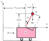 |
Fig. 1 Free body diagram of cart-inverted pendulum. |
3 Proposed controller design
The objective of a controller is to swing the pendulum from a stable pendant position to an unstable upright position and stabilize it there with minimum oscillations using less controller effort. Conventional control has given numerous methods to design controllers for dynamic systems, such as PID, state-feedback and observer-based, LQR-based, H2 or Hꝏ, etc., to address a wide range of applications in the science and engineering domain. Conventional PID controllers are still the most implemented controllers in the literature because of their simplicity, reliability, and ease of understanding, but they suffer from parameter tuning and stability issues in the presence of uncertainties [30–32], so this may not be sufficient to handle the complexity of the nonlinear CIP model. The fractional-order PID offers enhanced performance compared to the standard PID due to the inclusion of two additional tuning gains (μ, λ) in addition to the conventional PID gains (kp, kd, ki). They also combine the advantages of fractional-order calculus and the powerful PID technique. Cascaded FOPI-FOPD is another version of FOPID that has a series connection of fractional order proportional-integral block (lag controller for reduction) followed by a fractional order derivative block (lag controller to speed up response and provide desired stability margins) [26]. These individual control techniques give satisfying results while balancing the upright position of the pendulum, but it depends on the optimal controller parameter setting. They also perform poorly with model uncertainties and disturbances [33]. Unlike LQG, which is limited to linear systems, BLQGC can effectively control nonlinear systems and robustness to uncertainties and disturbances. BLQGC often demonstrates better accuracy and stability compared to traditional control methods like PID, fuzzy logic, and others.
Hence, the dynamism and complexity of the CIP model necessitate the integration of multiple control strategies. Hybridization of control techniques offers several advantages, like enhanced performance, improved adaptability, handling the nonlinearity efficiently, and increased reliability by mutually compensating for the limitations of individual methods. The proposed control method as depicted in Figure 2 takes advantage of both cascaded FOPI-FOPD and BLQGC techniques to achieve the desired performance. It has cascaded FOPI-FOPD technique as a feedback controller and BLQGC as a feedforward controller, respectively.
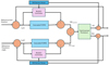 |
Fig. 2 The implemented cascaded FOPI-FOPD-BLQGC controlled CIP model. |
3.1 Cascaded FOPI-FOPD controller
To enhance system performance, this method combines the benefits of cascading the control elements with the ideas of fractional calculus in controller design. Cascaded FOPID controllers find application in mechanical systems, robotics, temperature control, and other technological disciplines that need precise control. Figure 3 shows various possible structures by changing μ and λ values.
The cascaded FOPI-FOPD controller structure (Fig. 4a) is different from conventional FOPID (Fig. 4b) as it connects the derivative controller and integral controller in series, whereas in FOPID, these controllers are connected in parallel. The results provided in the subsequent section indicate that this innovative structure offers enhanced robustness, stability, and transient performance. Equation (3) provides the controller gain for the suggested structure.
 (3)
(3)
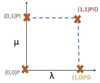 |
Fig. 3 Conversion of FOPID to conventional controllers. |
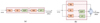 |
Fig. 4 (a) Proposed cascaded FOPI-FOPD controller and (b) conventional FOPID controller. |
3.2 Backstepping-linear quadratic Gaussian controller
Backstepping-linear quadratic Gaussian control (BLQG) is a powerful control design technique that effectively combines the advantages of backstepping and LQG. This method is particularly suited for nonlinear systems with uncertainties, offering superior performance compared to conventional control strategies. However, its computational complexity and reliance on accurate models should be considered when implementing it in real-world settings. The BLQG controller is widely employed in various fields where precise control is essential, even in the presence of uncertainties, such as aerospace, automotive, robotics, and process control. In contrast to the linear quadratic regulator (LQR) control method, which uses state feedback control based on the error between the reference and measured output, the BLQGC considers the error between the reference and estimated output. Due to its ability to adjust controller parameters based on predictions of system behavior, BLQGC outperforms LQR. Furthermore, the BLQGC can be designed for systems with unmeasurable states, as it estimates these states from its response to improve overall performance [34]. The BLQGC system incorporates a hybrid approach by integrating the Kalman estimator and LQR controller. This approach considers external disturbances and measurement noise as shown in Figures 5a,5b.
To control and stabilize the system, the BLQGC design considers the state-space model for a cart-inverted pendulum, which is discussed in Section 2. The state-space CIP model with output sensor or measurement noise D(t) and process disturbance F(t) has been taken into consideration in this design. A process disturbance signal F(t) is defined as a constant 1 N force applied to the cart, and an output state detection signal D(t) is defined as the appearance of white Gaussian noise. System states are estimated using the Kalman filter in advance to improve the system performance. The CIP state space model with additive white Gaussian noise and process disturbance is represented as equations (4–5).
 (4)
(4)
 (5)
(5)
where the variables xm(t) and u(t) represent the state and control input, respectively, while y(t) represents the measured output. Figure 5b illustrates the BLQGC design, which includes the LQR gain Kc and the backstepping gain controller gain Kb. To minimize the objective function given in equation (6), the Kc gain must be determined using equation (7).
 (6)
(6)
 (7)
(7)
where Q = CT qC, Q is positive semi-definite state weighting matrix and R is positive definite input weighting matrix. R and Q matrix are used to modify the control u(t) and system’s output: cart position and pendulum angle, and controller is tuned by changing these two matrixes to get desired response. The positive semi-definite matrix Π is obtained by solving the controller algebraic Riccati equation (CARE), given as in equation (8):
 (8)
(8)
Equations (9–11) gives the state-space of the CIP with estimated states by backstepping controller.
 (9)
(9)
where
 (10)
(10)
 (11)
(11)
So, equation (11) will get modified as equation (12).
 (12)
(12)
where Kb is backstepping controller gain, x(t) is estimated state vector, and ^ŷ(t) is estimated measured output vector. The Kb can be calculated as depicted as equation (13).
 (13)
(13)
where Πb is taken as positive definite matrix and can be formulated as solution of Lyapunov function, given in equation (14)
 (14)
(14)
where, (A – BKc) must be Hurwitz while calculating LQR gain Kc. I represent (n × n) identity matrix with n as the order of system matrix A, and Bd as the weighting matrix for measurement noise. Ultimately the BLQGC transfer function is derived using LQR gain and Kalman filter gain as shown in equation (15).
 (15)
(15)
Table 1 includes the estimated BLQGC controller parameters (Q, R, Q1, R1) used in this work, whereas Table 2 provides the estimated controller gains.
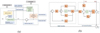 |
Fig. 5 (a) General BLQGC controller design, and (b) BLQGC controller design cart-inverted pendulum with state-space model. |
Proposed controller parameter values.
Proposed controller gain values.
4 Hybrid (GOA-FA) algorithm
The grasshopper optimization algorithm (GOA) and firefly algorithm (FA) are both nature-inspired metaheuristic algorithms used for optimization problems. GOA draws inspiration from the behavior of grasshoppers in a swarm, while FA mimics the bioluminescence of fireflies. GOA balances exploration and exploitation well, but there is a chance it might get stuck in local optima (sub-optimal solutions), so the hybridization with FA’s local search could help escape these traps and find the globally optimal solution. On the other hand, FA alone might struggle with the complexity of the cart-inverted pendulum system, especially for real-time control. Thus, GOA’s exploration abilities can help FA to explore the search space more efficiently. As a result, they can work together to attain the optimal control solution more quickly. The hybridization of GOA and FA excels at balancing exploration and exploitation. This is crucial for the cart-inverted pendulum system, which requires both finding the optimal control strategy and fine-tuning it for precise balancing.
Phase 1: Grasshopper optimization algorithm (GOA
The grasshopper optimization algorithm was proposed by Sareemi in 2017. The swarm life cycle goes through three phases: egg, nymph, and adulthood, but the important phases to determine the grasshopper’s life span are nymph and adulthood. The nymph depicts immature agents having slow movement and small steps, while the adulthood phase witnesses the aggressive nature of the swarm having longer steps and randomized movement in all directions in search of the best. These two phases of seeking food can be accomplished by exploration-nymph as well as exploitation-adulthood, which are mathematically modeled as follows [35,36]. The current location of grasshopper is modeled as equation (16).
 (16)
(16)
where L(i) depicts the ith grasshopper location, So(i) and Gf(i) are communal interaction as well as the gravity force on the ith grasshopper, correspondingly, and Aw(i) signifies wind advection.
Phase 2: Firefly algorithm
The firefly algorithm is a metaheuristic optimization algorithm that gives 78% to 86% of computational cost savings as compared to other well-known algorithms like PSO, GA, etc. because of automatic population subdivision, natural capability to deal with multimodal optimization, and high ergodicity and diversity in its solution [37,38]. This algorithm mainly models the attractiveness between current and subsequent flies in a forward direction. This attractiveness decreases with the increase in distance between flies and increases with the increase in brightness level of flies. Flies follow the random walk if the brightness of two flies is equal to uniform or nonuniform step size. So, new positions could model as a function of current position, brightness level, and random walk step size. This algorithm has two loops to generate the new solution: Inner loop for population size “n” and outer loop for number of iterations “t”. Complexity of algorithm is linear (n × t) for a smaller population and is nonlinear (n × log (nt)) for a larger population. Initial population will be generated according to the equations (17–18).
 (17)
(17)
 (18)
(18)
Flies new position to will between ith and jth location be modified based on brightness criterion and updated according to the position equations (19–20).
 (19)
(19)
 (20)
(20)
where α is random number between 0 and 1; εi(t) is a random variable drawn from uniform distribution, Gaussian distribution, or any other distribution form; and β0 is attractiveness control function mostly taken as 1.
Finally, by combining above discussed algorithm, the implemented hybrid (GOA-FA) algorithm is depicted below:
Hybrid GOA-FA algorithm
Define Parameters (Number of grasshoppers (h), Number of fireflies, Maximum number of iterations, Dimension of the problem (number of parameters to tune), Lower bound of parameter values, Upper bound of parameter values, Step size factor for grasshopper update, Light absorption coefficient for firefly update).
Initialize the grasshopper’s position and fireflies’ position randomly.
Main loop will have two phases of GOA and FA algorithm.
for t = 1:tmax
% Grasshopper algorithm loop begins%
for i = 1:num_grasshoppers
% Calculate the fitness function for each grasshopper%
Fitness _ grasshopper = evaluate _ fitness (grasshoppers _ position (i, :));
% Update position of grasshopper%
r = unifrnd (-α, α, 1, dim);% Randomization factor
grasshoppers _ position (i, :) = grasshoppers _ position (, :) + r.* (global _ best _ solution – grasshoppers _ position (i, :)).
% Apply boundary constraints
%Grasshoppers _ position (i, :) = max (min (grasshoppers _ position (i, :), ub), lb);
end
% Firefly Algorithm loop%
for i = 1:num_fireflies
% Calculate the fitness for each firefly%
Fitness _ firefly = evaluate _ fitness (fireflies _ position (I, :));
% Update position of firefly%
for j = 1:num_fireflies
if fitness _ firefly < evaluate _ fitness (fireflies _ position (j, :))
r = norm (fireflies _ position (i, :) – fireflies _ position (j, :))^2;
fireflies _ position (i, :) = fireflies _ position (I, :) + beta / r^2 * (fireflies _ position(j, :) – fireflies _ position(i, :))
% Apply boundary constraints%
fireflies _ position (i, :) = max (min (fireflies _ position (i, :), ub), lb);
End
End
% Return the optimal solution found%
disp(['Optimal Solution (Grasshopper): ', num2str(global_best_solution)]);
disp(['Optimal Fitness (Grasshopper): ', num2str(global_best_fitness)]);
5. Results and discussions
The capability and effectiveness of the suggested cascaded FOPI-FOPD-BLQGC controller are examined in this section. The implemented Cascaded FOPI-FOPD-BLQGC controlled CIP model is depicted in Figure 2. The CIP control needs the fast responses to maintain balance and removal of steady-state error for perfect balancing. The ITAE criterion reduces the time-weighted absolute error. It heavily penalizes the errors those exists for longer period and helps achieving enhanced stability and reduced oscillations. Thus, the ITAE (Integral time Absolute error) criterion is assumed as cost function JITAE and is calculated as equation (21).
 (21)
(21)
The hybrid Grasshopper and Firefly optimization algorithms (GOA-FA) is employed to search the optimal parameters, to achieve high stability and error handling for the proposed controller displays the adjusted cascaded FOPI-FOPD controller parameters using the hybrid (GOA-FA) optimization method. The comparative tunned parameters of all controllers are summarized in Table 3.
The transient performance analysis, stability analysis, and robust analysis of parametric uncertain CIP system subjected to impulse disturbance is compared for FOPI, FOPD, and BLQGC methods by evaluating rise time (tr), settling time (ts), maximum peak overshoot (Mp), and steady-state error (ess) parameters.
Tuned controller parameters.
5.1 Transient performance analysis
The transient analysis gives information about how the system reacts to disruptions or setpoint modifications. The comparative performance analysis of the proposed controller with FOPD, FOPI, and BLQGC controllers has been analyzed for pendulum angle, cart position, and controller effort responses as shown in Figures 6a–6c and quantitatively interpreted in Table 4. This analysis is carried out on the basis of tr, ts, Mp, and ess parameters.
This has been observed from Figure 6a that the pendulum-angle response results in ess values of 0, 0.05, 0.05, and 0.07 and ts values of 3, 13, 19, and 20 s with the proposed cascaded FOPI-FOPD-BLQGC, FOPD, FOPI, and BLQGC controllers, respectively. Further, Mp values obtained are 1.3, 0.4, 0.5, and 0.7 and tr values are 0.1, 0.4, 0.5, and 0.7 s, respectively, for these controllers. Similarly, from Figure 6b, ess values obtained for cart position are 0, 0.05, 0.05, and 0.07 and ts values are 3.2, 19, 19, and 20 s, respectively, for the above-said controllers. Further, Mp values obtained are 0.3, 0.8, 0.8, and 0.7 and tr values are 0.2, 0.5, 0.6, and 0.7s, respectively, for these controllers. Thus, the proposed hybrid controller results in the best ess, ts, Mp and tr values, as also shown in Table 4. The control signals for different controllers considered are shown in Figure 6c. The control signal for the proposed cascaded FOPI-FOPD-BLQGC exhibits a relatively smooth response with minimal overshoot and settling time in comparison to other controllers. The FOPI shows a more oscillatory response, indicating a less stable behavior compared to the proposed controller. The FOPD controller exhibits significant overshoot and undershoot and takes a longer time to settle compared to the other controllers. The BLQGC controller shows a relatively smooth response but with a slower settling time compared to the proposed control scheme. It also exhibits the overshoot and undershoots, indicating a less stable behavior than the cascaded controller. Hence, the proposed cascaded FOPI-FOPD-BLQGC controller is giving the least overshoot, undershoot, and settling time and minimum control effort as compared to FOPI, FOPD, and BLQGC controllers.
Thus, the best transient performance and control signal are given by the proposed cascaded FOPI-FOPD-BLQGC as compared to FOPD, FOPI, and BLQGC controllers.
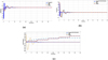 |
Fig. 6 Proposed (BLQGC- FOPID-FOPI) controller response tuned with GH-FA algorithm. (a) Pendulum angle response. (b) Cart position response. (c) Controller effort response. |
Comparative transient analysis.
5.2 Closed-loop stability analysis under impulsive disturbances
Stability is a crucial aspect to consider while designing any system, as an unstable system can result in adverse behavior, ranging from poor performance to system damage. This is particularly important when designing systems with life-critical applications, such as spacecraft, underwater vehicles, and human-driven transportation. In this work, an external force of 1 N was applied to the pendulum arm, causing a deviation in the pendulum angle, and the proposed controller is used to stabilize the pendulum in an upright position. Figures 7a–7c depicts the stability response of the pendulum angle, cart position, and controller effort. The CIP can recover from the disturbance and attain an upright position within 3.5 s. Furthermore, with the aid of the proposed controller, the cart returns to its reference position in 3.2 s, demonstrating satisfactory performance despite the sudden disruption.
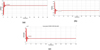 |
Fig. 7 Stability response of proposed controller with application of 1 N impulse force. (a) Pendulum angle response. (b) Cart position response. (c) Controller effort. |
5.3 Robustness analysis under parametric uncertainties
Robust analysis of any controller plays a crucial role in controller designing, as it ensures the satisfactory behavior of the model even in the presence of uncertainties. The pendulum mass (m) variation could modify the torque requirement to swing and stabilize the pendulum in an upright position. A change in cart mass (M) could be a result of a modified system parameter or disturbance parameter by giving an additional weight on the cart during the operation. And this will alter the external input force requirement. Similarly, pendulum length (l) will affect the total torque experienced by the pendulum and ultimately results in angle displacement [26–28]. So, it explains the interdependency of pendulum mass, cart mass, and pendulum length and their importance in any controller design. To evaluate the robustness of the proposed controller, three varied sets of cart mass (2.1–2.3 kg), pendulum mass (0.1–0.3 kg), and pendulum length (0.1–0.3 m) are considered as demonstrated in Cases 1–3 in the following section.
Case 1: The system parameters are changes to  , and l = 0.1 m (73.68 %) from the initial values, and its pendulum angle and cart-position responses are shown in Figurea 8a–8b and quantitatively compared in Table 5.
As shown in Table 5, tr time obtained with the proposed controller, FOPD, FOPI, and BLQGC are 0.1, 1.5, 1.8, and 2.0 s, respectively, to stabilize the pendulum and 0.1, 1.6, 1.7, and 2.0 s, respectively, for cart-position control. Similarly, Mp recorded for these controllers are 0.8, 0.2, 0.2, and 0.18, respectively, for pendulum control and 0.1, 0.3, 0.3, and 0.2, respectively, for cart-position control. Further, the proposed controller also attained the zero ess value in 2 s of ts time for both pendulum stabilization and cart stabilization. The FOPD, FOPI, and BLQGC controllers are settling to ess values of 0.06, 0.05, and 0.07 for pendulum angle and of 0.05, 0.05, and 0.07 for cart position in 20, 19, and 20 s of ts time, respectively. The results show that the implemented controller can stabilize the CIP with minimum values of tr, ess, Mp, and ts.
Case 2: The system parameters are changes to  , and l = 0.2 m(47.36%), from the initial setting, and its pendulum angle and cart-position responses are given in Figures 9a–9b and interpreted in Table 6.
As given in Table 6, the proposed controller, FOPD, FOPI, and BLQGC are getting tr of 0.1, 2, 3, and 3 s, respectively, for pendulum angle and are 0.1, 3, 3, and 3 s, respectively, for cart position. The Mp recorded for these controllers is 0.3, 0.7, 0.8, and 0.3, respectively, for pendulum control and 0.5, 0.4, 0.6, and 0.7, respectively, for cart control. Similarly, the proposed controller reaches zero ess value in 3 s for pendulum stabilization as well as cart stabilization, while FOPD, FOPI, and BLQGC reach ess value of 0.05, 0.05, and 0.08 for pendulum control and of 0.07, 0.05, and 0.07 for cart control in 18, 19, and 20 s of settling time, respectively.
Case 3: The system parameters are changes to  , and l = 0.3 m (21.05%) from the initial setting, and its pendulum-angle and cart-position responses are given in Figures 10a–10b and interpreted in Table 7.
As shown in Table 7, the proposed controller is getting a zero ess value in 3 s, and FOPD, FOPI, and BLQGC is reaching ess values of 0.05, 0.05, and 0.07 in 19, 19, and 20 s of ts time, respectively, for both pendulum stabilization and cart stabilization. Further, the tr time for these controllers is 1, 7, 7, and 7 s, respectively, to stabilize the pendulum and 2, 7, 7, and 7 s, respectively, for cart control. Similarly, the Mp for these controllers is 0.6, 0.5, 0.5, and 0.7, respectively, for pendulum control and 0.3, 0.5, 0.5, and 0.7, respectively, for cart control. The results again confirm the superiority of the proposed cascaded FOPI-FOPD-BLQGC, as it is giving better values of tr, Mp, ts, and ess.
The responses portrayed through Figures 8–10 under prevailing test conditions of Cases 1–3 confirm the competency of the proposed cascaded FOPI-FOPD-BLQGC controller toward successful stabilization of CIP even in the presence of such parametric variations.
 |
Fig. 8 Comparative responses with M = 2.1 kg, m = 0.1 kg, l = 0.1 m. (a) Pendulum angle response. (b) Cart position response. |
Comparative transient parameters for Case 1.
 |
Fig. 9 Comparative responses with M = 2.1 kg, m = 0.3 kg, l = 0.3 m. (a) Pendulum angle response. (b) Cart position response. |
Comparative transient parameters for Case 2.
 |
Fig. 10 Comparative responses with M = 2.3 kg, m = 0.3 kg, l = 0.3 m. (a) Pendulum angle response. (b) Cart position response. |
Comparative transient parameters for Case 3.
5.4 Frequency domain analysis
Frequency domain parameters: gain margin (GM), phase margin (PM), and bandwidth (BW) are used for analyzing the proposed controller in comparison to other techniques. The magnitude and phase variation against frequency are depicted in Figure 11, and parameter values are summarized in Table 8. The GM and PM represent the maximum values of gain and phase up to which the system remains stable. The GM achieved with the proposed controller, FOPD, FOPI, and BLQGC are 8.02, 6.8, 6.5, and 6, respectively. Similarly, the PM and BW recorded with these controllers are 45, 45, 44, and 44 and 3.5, 3.3, 3.2, and 3.1, respectively. Hence, the improved frequency response of CIP with proposed controllers in terms of GM (8.02), PM (45), and BW (3.5) is confirmed over other controllers.
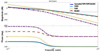 |
Fig. 11 Comparative Bode plot of proposed model. |
Frequency domain (Bode plot) parameters.
6 Conclusion
This paper presents a hybrid cascade FOPI-FOPD-BLQGC controller for ensuring stability and control of a cart-inverted pendulum. The design of the proposed controller involves the consideration of two distinct control loops to control the cart position and pendulum angle. The feedback loop utilizes a cascaded FOPI-FOPD control to generate the control signal. The BLQGC controller is linked in a feedforward loop to generate a control signal in the presence of white Gaussian noise. In addition, the hybrid GOA-FA artificial intelligence technique is employed for the automatic tuning of controller parameters. The proposed controller has shown substantial enhancements in transient analysis, stability, robust analysis, and robust analysis as compared to FOPD, FOPI, and BLQGC control methods under different parametric uncertain situations. The proposed cascade FOPI-FOPD-BLQGC controller offers greater resilience against parametric disturbances, excellent transient performances, and superior stability. These features make it suitable for real-time applications such as Segway, robotics, rockets, and missile guiding systems. In future work, the proposed controller will be applied to other CIP variants, such as the rotating and double inverted pendulum systems. The controller parameters will be further fine-tuned using advanced and emerging optimization techniques. In addition, extended robust studies will be carried out under wider operating conditions, parametric uncertainties, and external disturbances, including Pareto-based analysis to identify the wider robust design space. Rigorous Lyapunov-based stability analysis will also be performed to establish formal mathematical guarantees of closed-loop stability.
Funding
There is no funding for this study.
Conflicts of interest
There is no conflict of Interest for this study.
Data availability statement
There is no data availability for this study.
Author contribution statement
Conceptualization, Neelam Verma and Sudarshan K. Valluru; Methodology, Neelam Verma; Software, Neelam Verma; Validation, Neelam Verma and Sudarshan K. Valluru; Formal Analysis, Neelam Verma; Investigation, Neelam Verma; Resources, Neelam Verma; Writing—Original Draft Preparation, Neelam Verma; Writing—Review & Editing, Neelam Verma and Sudarshan K. Valluru; Supervision, Sudarshan K. Valluru.
References
- O. Boubaker, The inverted pendulum benchmark in nonlinear control theory: a survey, Int. J. Adv. Robot. Syst. 10, 1–10 (2013) [Google Scholar]
- K. Kaheman, U. Fasel, J.J. Bramburger, B. Strom, J.N. Kutz, S.L. Brunton, The experimental multi-arm pendulum on a cart: a benchmark system for chaos, learning, and control, HardwareX 15, 465 (2023) [Google Scholar]
- B. Bekkar, K. Ferkous, Design of online fuzzy tuning LQR controller applied to rotary single inverted pendulum: Experimental validation, Arab. J. Sci. Eng. 48, 6957–6972 (2023) [Google Scholar]
- S. Mishra, A. Arora, A Huber reward function-driven deep reinforcement learning solution for cart-pole balancing problem, Neural Comput. Appl. 35, 16705–16722 (2023) [Google Scholar]
- F. Peker, I. Kaya, E. Cokmez, S. Atic, Cascade control approach for a cart inverted pendulum system using controller synthesis method, in: Proceedings of the 26th Mediterranean Conference on Control and Automation 2018, pp. 1–6 [Google Scholar]
- C. Mahapatra, S. Chauhan, B. Hemakumar, Servo control and stabilization of linear inverted pendulum on a cart using LQG, in: Proceedings of the International Conference on Power, Energy, Environment and Intelligent Control, 2018, pp. 783–788 [Google Scholar]
- S.K. Mishra, D. Chandra, Stabilization and tracking control of inverted pendulum using fractional order PID controllers, J. Eng. 2014, 1–9 (2014) [Google Scholar]
- R. Ramakrishnan, D.S. Nachimuthu, Design of state feedback LQR based dual mode fractional-order PID controller using inertia weighted PSO algorithm for control of an underactuated system, J. Inst. Eng. (India) Ser. C 102, 1–12 (2021) [Google Scholar]
- K.M. Goher, S.O. Fadlallah, Control of a two-wheeled machine with two-directions handling mechanism using PID and PD-FLC algorithms, Int. J. Autom. Comput. 16, 511–533 (2019) [Google Scholar]
- V. Bassi, S.K. Mishra, E.E. Omizegba, Automatic tuning of proportional–integral–derivative (PID) controller using particle swarm optimization (PSO) algorithm, Int. J. Artif. Intell. Appl. 2, 25–34 (2011) [Google Scholar]
- K. Isik, G.C. Thomas, L. Sentis, A fixed structure gain selection strategy for high impedance series elastic actuator behavior, J. Dyn. Syst. Meas. Control 141, 021009 (2019) [Google Scholar]
- R. Banerjee, A. Pal, Stabilization of inverted pendulum on cart based on LQG optimal control, in: Proceedings of the International Conference on Computing for Sustainable Development, 2018, pp. 1–6 [Google Scholar]
- A.D. Kuo, An optimal control model for analyzing human postural balance, IEEE Trans. Biomed. Eng. 42, 87–101 (1995) [Google Scholar]
- C.A. Monje, Y.Q. Chen, B.M. Vinagre, D. Xue, V. Feliu, Fractional-order Systems and Controls. Fundamentals and Applications, Springer, London, 2010 [Google Scholar]
- M. Magdy, A. El Marhomy, M.A. Attia, Modeling of inverted pendulum system with gravitational search algorithm optimized controller, Ain Shams Eng. J. 10, 129–149 (2019) [Google Scholar]
- E.Y. Bejarbaneh, M. Masoumnezhad, D.J. Armaghani, B.T. Pham, Design of robust control based on linear matrix inequality and a novel hybrid PSO search technique for autonomous underwater vehicle, Appl. Ocean Res. 101, 102231 (2020) [Google Scholar]
- D.H. Al-Janan, H.C. Chang, Y.P. Chen, T.K. Liu, Optimizing the double inverted pendulum’s performance via the uniform neuro multiobjective genetic algorithm, Int. J. Autom. Comput. 14, 641–654 (2017) [Google Scholar]
- Z. Sun, N. Wang, Y. Bi, Type-1/type-2 fuzzy logic systems optimization with RNA genetic algorithm for double inverted pendulum, Appl. Math. Model. 39, 569–584 (2015) [Google Scholar]
- A.S. Al-Araji, An adaptive swing-up sliding mode controller design for a real inverted pendulum system based on Culture-Bees algorithm, Eur. J. Control 45, 1–9 (2019) [Google Scholar]
- S.J. Chacko, R.J. Abraham, On LQR controller design for an inverted pendulum stabilization, Int. J. Dyn. Control 11, 1584–1592 (2023) [Google Scholar]
- F.M. Escalante, A.L. Jutinico, M.H. Terra, A.A.G. Siqueira, Robust linear quadratic regulator applied to an inverted pendulum, Asian J. Control 25, 2564–2576 (2023) [Google Scholar]
- L. Wang, H. Ni, W. Zhou, P.M. Pardalos, J. Fang, M. Fei, MBPOA-based LQR controller and its application to the double-parallel inverted pendulum system, Eng. Appl. Artif. Intell. 36, 376–386 (2014) [Google Scholar]
- P. Dwivedi, S. Pandey, A.S. Junghare, Stabilization of unstable equilibrium point of rotary inverted pendulum using fractional controller, J. Franklin Inst. 354, 7754–7773 (2017) [Google Scholar]
- Z. Ben Hazem, M.J. Fotuhi, Z. Bingül, Development of a fuzzy-LQR and fuzzy-LQG stability control for a double link rotary inverted pendulum, J. Franklin Inst. 357, 10529–10556 (2020) [Google Scholar]
- C. Lei, R. Li, Q. Zhu, Design and stability analysis of semi-implicit cascaded proportional-derivative controller for underactuated cart-pole inverted pendulum system, Robotica 42, 87–117 (2024) [Google Scholar]
- R. Mondal, J. Dey, A novel design methodology on cascaded fractional order (FO) PI-PD control and its real time implementation to cart-inverted pendulum system, ISA Trans. 130, 469–480 (2022) [Google Scholar]
- N. Verma, S.K. Valluru, ANN based ANFIS controller design using hybrid meta-heuristic tuning approach for cart inverted pendulum system, Multimed. Tools Appl. 1–23 (2023) [Google Scholar]
- N. Verma, S.K. Valluru, Comparative study of parametric disturbances effect on cart-inverted pendulum system stabilization, Lect. Notes Electr. Eng. 948, 1–10 (2023) [Google Scholar]
- S.K. Valluru, M. Singh, M. Singh, V. Khattar, Experimental validation of PID and LQR control techniques for stabilization of cart inverted pendulum system, in: Proceedings of the IEEE International Conference on Recent Trends in Electronics, Information and Communication Technology (RTEICT), Bangalore, India, 2018, pp. 708–712. [Google Scholar]
- S.M. Schlanbusch, J. Zhou, Adaptive backstepping control of a 2-DOF helicopter system with uniform quantized inputs, in: Proceedings of the IECON–Industrial Electronics Conference, 2020, 1–6 [Google Scholar]
- T. Pangaribuan, M.N. Nasruddin, E. Marlianto, M. Sigiro, The influences of load mass changing on inverted pendulum stability based on simulation study, IOP Conf. Ser. Mater. Sci. Eng. 237, 012005 (2017) [Google Scholar]
- S.K. Valluru, M. Singh, Performance investigations of APSO tuned linear and nonlinear PID controllers for a nonlinear dynamical system, J. Electr. Syst. Inf. Technol. 5, 653–663 (2018) [Google Scholar]
- R. Mondal, J. Dey, Performance analysis and implementation of fractional order 2-DOF control on cart-inverted pendulum system, IEEE Trans. Ind. Appl. 56, 7055–7066 (2020) [Google Scholar]
- A.K. Patra, S.S. Biswal, P.K. Rout, Backstepping linear quadratic Gaussian controller design for balancing an inverted pendulum, IETE J. Res. 68, 88–100 (2022) [Google Scholar]
- L. Abualigah, A. Diabat, A comprehensive survey of the Grasshopper optimization algorithm: Results, variants, and applications, Neural Comput. Appl. 32, 15529–15557 (2020) [Google Scholar]
- N. Verma, S.K. Valluru, Comparative analysis of GOA, WCA and PSO tuned fractional order-PID controller for cart-inverted pendulum, in: Proceedings of the IEEE International Power and Renewable Energy Conference, Kollam, India, 2022, pp. 1–6 [Google Scholar]
- A.H. Saleh, S.A. Al-khafaji, Anti-swing rejection based on PID controller optimized by firefly algorithm, Math. Model. Eng. Probl. 10, 178–184 (2023) [Google Scholar]
- I. Jarraya, L. Degaa, N. Rizoug, M.H. Chabchoub, H. Trabelsi, Comparison study between hybrid Nelder–Mead particle swarm optimization and open circuit voltage–recursive least square for the battery parameters estimation, J. Energy Storage 50, 104424 (2022) [Google Scholar]
Cite this article as: N. Verma, S. K. Valluru, Design of cascaded FOPI-FOPD-BLQG controller tuned with hybrid grasshopper and firefly algorithms for stabilizing cart-inverted pendulum system, Mechanics & Industry 27, 14 (2026), https://doi.org/10.1051/meca/2026009
All Tables
All Figures
|
Fig. 1 Free body diagram of cart-inverted pendulum. |
| In the text | |
|
Fig. 2 The implemented cascaded FOPI-FOPD-BLQGC controlled CIP model. |
| In the text | |
|
Fig. 3 Conversion of FOPID to conventional controllers. |
| In the text | |
|
Fig. 4 (a) Proposed cascaded FOPI-FOPD controller and (b) conventional FOPID controller. |
| In the text | |
|
Fig. 5 (a) General BLQGC controller design, and (b) BLQGC controller design cart-inverted pendulum with state-space model. |
| In the text | |
|
Fig. 6 Proposed (BLQGC- FOPID-FOPI) controller response tuned with GH-FA algorithm. (a) Pendulum angle response. (b) Cart position response. (c) Controller effort response. |
| In the text | |
|
Fig. 7 Stability response of proposed controller with application of 1 N impulse force. (a) Pendulum angle response. (b) Cart position response. (c) Controller effort. |
| In the text | |
|
Fig. 8 Comparative responses with M = 2.1 kg, m = 0.1 kg, l = 0.1 m. (a) Pendulum angle response. (b) Cart position response. |
| In the text | |
|
Fig. 9 Comparative responses with M = 2.1 kg, m = 0.3 kg, l = 0.3 m. (a) Pendulum angle response. (b) Cart position response. |
| In the text | |
|
Fig. 10 Comparative responses with M = 2.3 kg, m = 0.3 kg, l = 0.3 m. (a) Pendulum angle response. (b) Cart position response. |
| In the text | |
|
Fig. 11 Comparative Bode plot of proposed model. |
| In the text | |
Current usage metrics show cumulative count of Article Views (full-text article views including HTML views, PDF and ePub downloads, according to the available data) and Abstracts Views on Vision4Press platform.
Data correspond to usage on the plateform after 2015. The current usage metrics is available 48-96 hours after online publication and is updated daily on week days.
Initial download of the metrics may take a while.