| Issue |
Mechanics & Industry
Volume 19, Number 1, 2018
|
|
|---|---|---|
| Article Number | 106 | |
| Number of page(s) | 15 | |
| DOI | https://doi.org/10.1051/meca/2017017 | |
| Published online | 31 August 2018 | |
Regular Article
Numerical and experimental study of a jet impinging with axial symmetry with a set of heat exchanger tubes
1
Department of Mechanical Engineering, Germi Branch, Islamic Azad University,
Germi, Iran
2
Department of Renewable Energies, Faculty of New Science & Technologies, University of Tehran,
Tehran, Iran
3
Department of Materials Science and Engineering, Sharif University of Technology,
Tehran, Iran
4
Faculty of Mechanical Engineering, Shahrood University of Technology,
Shahrood, Iran
* e-mail: This email address is being protected from spambots. You need JavaScript enabled to view it.
, e-mail: This email address is being protected from spambots. You need JavaScript enabled to view it.
Received:
9
October
2016
Accepted:
16
March
2017
Abstract
The main purpose of this research is to predict the flow field of impinging turbulent jet with cylinder in a 3-d state. Nowadays, shear stress has multiple uses in the industry. The study has been conducted in both compressible and incompressible states with output velocities between 100 and 150 m/s, in different eccentricities of jet with respect to the first cylinder, and in various nozzle outlet orifice distances from front edge of the first cylinder. Pressure distribution and shear stress on cylinder surfaces have been determined and efficiency of jet in cleaning the heat exchangers pipes has been analyzed. Also, an experimental investigation has been conducted in order to verify the accuracy of the numerical results. Results show that if the distance between nozzle outlet orifice and the front edge of the first cylinder (L) equals 1.52 D (D is the diameter of the cylinder), the jet has the highest cleaning effect.
Key words: Impinging turbulent jet / compressible 3D flow / hydrodynamic analysis / cylinder / turbulence model
© AFM, EDP Sciences 2018
1 Introduction
In 1992, the impinging of laminar jet with a cylinder was studied [1]. In 1996, the impinging of turbulent jet with a circular cylinder was also studied. In this study, the optimal distance from the cylinder to obtain the maximum level of cleaning, and the position of the separation points in states with eccentricity and without eccentricity, obtained theoretically and experimentally [2].
Also, in 1998, a impinging of two dimensional turbulent jet with a cylinder was studied at different eccentricities using various turbulence models [3]. In the same year, impinging of two dimensional turbulent jet with two cylinders, which was relative to the cylinder axis with a 45-degree angle, was studied [4]. Another researcher in 2000 examined numerically and experimentally the collision of two-dimensional turbulent jet with two parallel cylinders [5]. In 2001, one of the researchers studied the collision of a jet with axial symmetry with a cylinder in the direction of the perpendicular to the cylinder axis and studied numerically and experimentally at the various eccentricities. He concluded that in the state of L = 2.51 D, jet has the most cleaning effect [6].
In the present work, the impact of a jet with axial symmetry with four cylinders in the direction perpendicular to the axis of the first cylinder and in the different eccentricities to the first cylinder is numerically and experimentally studied. The main advantage of this study is that the flow field is three-dimensional and the effect of the cylinders on the cleaning of the other cylinder surfaces has been studied.
In this paper, high speed jets are considered, which they can be used as separating jets. The main purpose of this work is to analyze the efficiency of jet in cleaning the surfaces, particularly the surfaces of heat exchangers pipes. Heat exchangers are devices that provide heat transfer between two fluids with different temperatures, which are separated by a solid wall. Heat exchangers have applications in building heating systems, air conditioners, plants, petroleum industries, waste heat recovery, and chemical processes.
In using heat exchangers, after a working period, heat transfer surfaces are covered by sediments caused by fluids of the system. These sediments cause an additional heat resistance, which may decrease the performance of the heat exchanger to half of its initial value. Therefore, the quality of cleaning the heat transfer surfaces is of importance for performance recovery of the exchanger. The aim of cleaning effect is the amount of shear stress on the surface of cylinders.
Usually, the fluid that has a tendency to precipitate is considered inside the exchanger pipes; because high velocity and smooth surfaces reduce the formation rate of the sediment layer, but if the conditions and factors in the design of the exchanger cause the fluid to flow on the outer side of the outer shell, a mechanical cleaning method is used to remove sediments.
2 Governing equations of fluid flow
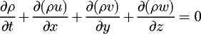
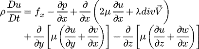
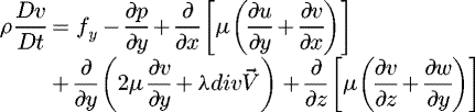
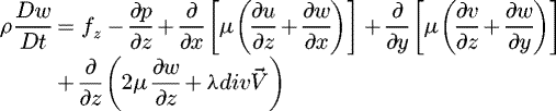
The equations governing fluid flow are the three equations of conservation or transfer, which can be briefly stated as:
 (1)
(1)
 (2)
(2)
 (3)
Equation (1), is a continuum equation that derives from the conservation principle of mass, equation (2), are the Navier-Stokes equations derived from the conservation principle of momentum and equation (3), is an energy equation that results from the conservation principle of energy.
(3)
Equation (1), is a continuum equation that derives from the conservation principle of mass, equation (2), are the Navier-Stokes equations derived from the conservation principle of momentum and equation (3), is an energy equation that results from the conservation principle of energy.
Turbulent flows are determined by fluctuating velocity field. Continuity equation and Navier-Stokes equations with unsteady term are momentarily true for turbulent flows. In the turbulent flow, every quantity, like ϕ, contains average and fluctuating components, where the average component is independent of time, but the fluctuating component depends on time. Therefore, it can be stated as:
 (4)
Here, the quantity of ϕ can be velocity, pressure, temperature or every other desirable quantity. Such as:
(4)
Here, the quantity of ϕ can be velocity, pressure, temperature or every other desirable quantity. Such as:
 Now, if the continuity equation in the incompressible fluid is considered, taking average of the total equation results in:
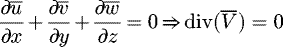 (5)Then, if (5) be subtracted from the main equation (momentary), it can be shown as:
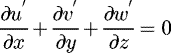 (6)Therefore, the continuity equation is separately true for both the average and fluctuating components. But, if the fluid is compressible, the aforementioned content cannot be true. Because the expressions containing
  , relate the two equations to each other. We mainly consider (5).
In order to obtain momentum equation in the state of turbulent flow, Navier-Stokes equations for incompressible fluid are considered; instead of u, v, w, p and f, average and fluctuating components are used; and time average is taken from the total equation. Regarding that (6) is true, equations below can be written.

 (7)
(7)
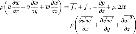 The left sides of equations in (7) are like Navier-Stokes equations for laminar flow, where instead of u, v, w, the quantities
  ,
,  ,
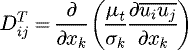
,  are used. The pressure and friction expressions in the right side of equations are also similarly changed. The additional expressions appeared in the equations are due to turbulent fluctuating motions. This component can be defined as a stress tensor as below:
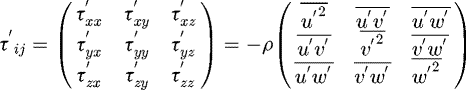 (8)The above stress tensor is called Reynolds stress tensor and the equations in (7) are called Reynolds equations in turbulent flow.
3 Turbulence models
A turbulence model is a computational procedure for making a system of average flow equations so that about a wide range of flow problems can be solved. In the two-equation models, two-equation of transfer, the partial differential equation is solved for turbulence kinetic energy k in one of the equations, and for the rate of dissipation of turbulence kinetic energy ϵ in the other [7]. From the four turbulence models to be mentioned in the following sections, the first three models are two-equation, and the last one is seven-equation.
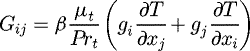
In the transfer equations of k-ε models, Gk is the generation of turbulence kinetic energy caused by average speed gradients; Gb is the generation of turbulence kinetic energy caused by buoyancy effects; and Ym shows the effect of fluctuating expansion on compressible turbulence with total rate of dissipation. The calculation of each of the above-mentioned parameters is shown as follow:
 (9)
where S is the absolute value of average strain rate tensor and is obtained as
(9)
where S is the absolute value of average strain rate tensor and is obtained as  . Sij is obtained as below:

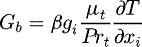 (10)where Prt is turbulent Prandtl number for energy. For the standard and realized k-ε models, the value of Prt equals 0.85; and for the k-ε RNG models, it is obtained as
  (α is inverse effective Prandtl number). β is the thermal expansion coefficient, which is defined as
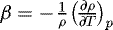
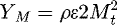 (11)where Mt is the turbulent Mach number and is defined as
  .
.  is the speed of sound [8].
3.1 Standard k-ε model
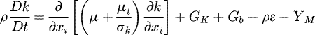
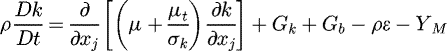
This model is a two-equation and semi-experimental model based on equations of transfer model for the turbulence kinetic energy k, and rate of dissipation ε, which has been proposed by Jones and Launder [9]. In its extraction two important conditions are considered: 1) the flow must be completely turbulent and 2) molecular viscosity effects must be negligible. This model has an acceptable accuracy for industrial flows; its pros and cons are completely obvious; and has wide application in the industry. Transfer equations for k and ε are as follow:
 (12)
(12)
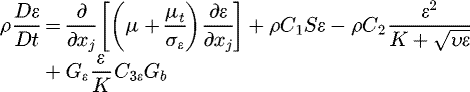
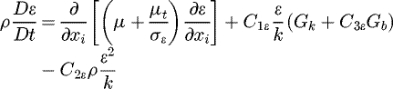 (13)
where Gk is the generation of turbulence kinetic energy caused by gradients of average velocity, Gb is the generation of turbulence kinetic energy caused by buoyancy effects and Ym is fluctuation expansion effect in compressible turbulence with total rate of dissipation. Calculation of the above parameters has been mentioned in the previous section. C1ε, C2ε, C3ε are constant values and σk and σε are turbulent Prandtl numbers for k and ε, respectively.
(13)
where Gk is the generation of turbulence kinetic energy caused by gradients of average velocity, Gb is the generation of turbulence kinetic energy caused by buoyancy effects and Ym is fluctuation expansion effect in compressible turbulence with total rate of dissipation. Calculation of the above parameters has been mentioned in the previous section. C1ε, C2ε, C3ε are constant values and σk and σε are turbulent Prandtl numbers for k and ε, respectively.
Turbulent or eddy viscosity, µt, is calculated combining k and ε as follows:
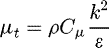 (14)
where Cµ is a constant value.
(14)
where Cµ is a constant value.
The constant values of this model are given in Table 1.
Constant values of standard k-ε model.
3.2 RNG k-ε modeling
This model is obtained applying a difficult statistical method (called group theory of re-nondimensionalizing). This model is similar to standard k-ε model in terms of structure, but also contains the following modifications:
-
RNG model has an additional expression in the equation of ε, which improves the accuracy especially for the flows with rapid strain;
-
In this model, the effect of rotation on turbulence is considered, which enhances the accuracy for rotational flows;
-
RNG theory gives an analytical formula for turbulent Prandtl numbers, whereas standard k-ε model uses specified constant values;
-
While standard k-ε model is a model with high Reynolds number, RNG theory gives a differential equation for effective viscosity, which is obtained analytically and considers effects of low Reynolds numbers. Though, effective use of this property depends on an appropriate treatment of the near-wall area.
These properties have caused this model, compared to standard k-ε model, to be accurate and logical for wide variants of flows. A comprehensive explanation of RNG theory and its application in turbulence have been given in [10].
The transfer equations for k and ε, in this model, are given as follow:
 (15)
(15)
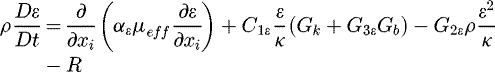 (16)
where Gk, Gb and Ym are as the quantities presented for standard k-ε turbulence model. αk and αε are inverse effective Prandtl numbers for k and ε, respectively.
(16)
where Gk, Gb and Ym are as the quantities presented for standard k-ε turbulence model. αk and αε are inverse effective Prandtl numbers for k and ε, respectively.
These quantities, using RNG theory, are obtained as follows:
 (17)
where α0 = 1.0. In limit state with high Reynolds number
(17)
where α0 = 1.0. In limit state with high Reynolds number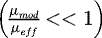 , we have αk = αϵ ≈ 1.393.
The process of scale elimination in RNG theory, leads to a differential equation for turbulent viscosity as follows:
 (18)
where
(18)
where  and Cυ ≈ 100.
In order to obtain the quality of effective turbulent transfer change with effective Reynolds number (with eddy scale), (18) is integrated, therefore, this model can be used satisfactorily for the flows with low Reynolds number and the flows in the near-wall. The limit state, i.e. high Reynolds number, leads to  , where using RNG theory, the value Cμ = 0.0845 is obtained. It is observable that this value is very close to the experimental value obtained for Cµ in standard k-ε model as 0.09.
The main difference of this model with standard k-ε model is in the R expression, which is obtained as follow:
 (19)
where
(19)
where  , η0 = 4.38 and β = 0.012. The constants of this model are given in Table 2.
The constants of RNG k-ε turbulence model.
3.3 Realizable k-ε model
The realizable k-ε model is a rather recently developed model and has two main differences with standard k-ε model:
-
the realizable k-ε model has a new formulation for turbulent viscosity;
-
in this model, from a precise and complete equation for square average transfer of eddy fluctuation, a new transfer equation for the rate of dissipation of ε has been obtained.
This model was proposed by Shih et al. [11]. The transfer equations of this model for k and ε are as follow:
 (20)
(20)
 (21)
where
(21)
where 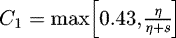 and
and  . Gk, Gb and Ym are as the quantities presented for standard k-ε turbulence model. C1ε, C2ε, C3ε are constant values and σk and σε are Prandtl numbers for k and ε, respectively.
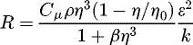
This model is valid for a wide range of flows such as homogeneous shear and rotational flows, free flows like jets and mixing layers, canal flows and boundary layer, and separation flows [11,12]. In realizable k-ε model, the turbulent viscosity is modeled as in the standard k-ε model and RNG model. The only difference is in the factor Cµ, which is not constant here and is obtained as follows [13]:
 (22)
where
(22)
where
 where
where  and
and  .
.  is the average tensor of rotation intensity in a rotational framework with angular velocity as ωk. Constants of the model, A0 and As, are obtained as:


 It can be observed that Cµ is a function of average strain rate, average rotation rate, angular velocity of system's rotation and turbulence fields (k and ε). The constants of this model are given in Table 3 [11].
Constants of realizable k-ε turbulence model.
3.4 Reynolds stress model (RSM)
This model strictly takes into account the effects of line curvature in flow, circulation, rotation and immediate changes in the intensity of strain. Compared to one-equation and two-equation models, this model has great capability in the accurate prediction of complex flows. This model has good efficiency in tornado flows, high circulation flows in combustion chambers, rotational flows in crossings and secondary flows excited by stress in tubes.
Transfer equations of Reynolds stresses,  , can be stated as follow [8–10]:
 (23)
where Cij,
(23)
where Cij,  , Pij and Fij do not require to be modeled, but
  , Gij, Φij and ϵij must be modeled.
Using scalar turbulent diffusion, turbulent diffusion transfer,  , is simplified as follow [18]:
 (24)
Turbulent viscosity µt is obtained from
(24)
Turbulent viscosity µt is obtained from 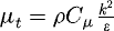 . Lien and Leschziner have obtained the value σk = 0.82 in [18].
Considering the proposals by Gibson and Launder [14], Fu et al. [19], and Launder [15,20] the pressure strain term ϕij can be separated and modeled as:
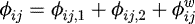 (25)
where ϕij,1 is slow pressure strain term (return to homogeneous state term); ϕ,ij,2is rapid pressure strain term; and ϕωis wall reflection term and are modeled as follow:
(25)
where ϕij,1 is slow pressure strain term (return to homogeneous state term); ϕ,ij,2is rapid pressure strain term; and ϕωis wall reflection term and are modeled as follow:
 (26)where C1 = 1.8.
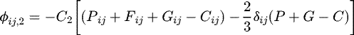 (27)where C2 = 0.6. Pij, Fij, Gij and Cij are defined as shown in (23) and some quantities are defined as
  ,
,  and
and  .
.
 (28)where
  ,
,  , nk is k-th component of unity normal vector, perpendicular to wall, d is vertical distance to wall and
  in which Cμ = 0.09 and κ = 0.41. This term is valid for re-distribution of vertical stresses near the wall and tends to decrease the stress perpendicular to wall and increase the stresses parallel to wall. Generation expressions caused by buoyancy effects are modeled as follows:
 (29)where Prt is turbulent Prandtl number for energy and it equals to 0.85.
The turbulence kinetic energy, considering trace of Reynolds stress tensor, is calculated as follows:
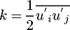 (30)
In order to obtain boundary conditions for Reynolds stresses, the transfer equation for turbulence kinetic energy is extracted as below:
(30)
In order to obtain boundary conditions for Reynolds stresses, the transfer equation for turbulence kinetic energy is extracted as below:
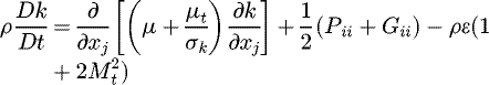 (31)where σk = 0.82. Although the above equation is solved generally for the whole domain of flow, the values obtained for k are used just in boundary conditions. In other conditions, k is obtained from (30).
Tensor of dissipation ϵij is modeled as:
 (32)
where
(32)
where 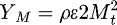 is an additional term as expansion dissipation [21] and Mt is turbulent Mach number. The scalar quantity of rate of dissipation ε is obtained as follows:
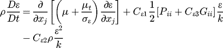 (33)where σϵ = 1.0, Cϵ1 = 1.44, Cϵ2 = 1.92 and Cϵ3 is a function of local flow direction with respect to gravitational vector.
3.5 The treatment of near-wall for turbulent flows surrounded by wall
In order to analyze near-wall treatment the non-equilibrium wall functions and logarithmic law of average velocity sensitive to pressure gradient are used, which are as follow:
 (34)
(34)
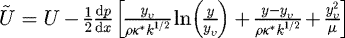 (35),
(35), 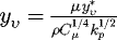
where yυ is physical viscous sub-layer thickness and 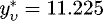 .
.
In order to calculate the generation and the dissipation of the turbulence kinetic energy in near-wall elements, the non-equilibrium wall function uses the concept of two-layer which is required in solving equation k in near-wall elements. It is assumed that the near-wall elements include viscous sub-layer and fully turbulent layer. For turbulence quantities, the following profile assumption is applied:
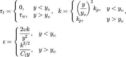 (36)
where
(36)
where 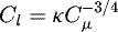 and yυ is viscous sub-layer non-dimension thickness. Applying these assumptions, average generation (k) of element (
 ) and average dissipation rate of element (
 ) can be obtained from volumetric average of Gk and ϵ of near-wall elements. For quadrilateral and hexahedral elements, volumetric average is obtained as:
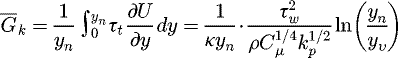 (37)
(37)
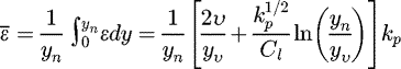 (38)where yn is the height of element defined as (yn = 2yp). For the elements with other shapes (such as triangular and four-dimensional elements) appropriate volumetric averages are utilized.
In (37) and (38), generation and dissipation of turbulence kinetic energy for near-wall elements are sensitized effectively to the proportion of viscous sub-layer and fully turbulent layer which is widely changed from an element to other in the high non-equilibrium flows. It effectively undermines the assumption of local equilibrium (dissipation = generation), which is considered by standard wall functions in calculation of generation and dissipation of turbulence kinetic energy in near-wall elements. In fact, non-equilibrium wall functions, to some extent, consider neglected non-equilibrium effects of standard wall functions in calculations. Therefore, in complex flows, when the average flow and turbulence are subjected to severe pressure gradients and rapid changes and the flow contains separation, reattachment, and impingement, it is better to use non-equilibrium wall functions.
4 Numerical model
In this work, diameter of nozzle outlet orifice is d = 0.0125 m (0.5 inch), diameter of cylinders D = 0.0254 m (1 inch) and length of cylinders is 40 cm. Exit air velocity from nozzle in different stages is considered between 100 and 150 m/s and the flow of jet is in stable state. For the above nozzle velocities and assuming the sound velocity in air as 343.2 m/s, in ambient temperature as 20∘C, the Mach number of output flow from nozzle is obtained according to Table 4, where in the analyses it is assumed that the flow is incompressible in velocity range of 100–120 m/s and it is compressible in the velocity range of 130–150 m/s.
In the study of impinging jets, the critical Reynolds number is calculated based on diameter of nozzle and its output velocity. This number for axis symmetric jets is in the range of 3000–14000, where in this study the calculated Reynolds number, based on output velocity as 100 m/s, is about 71000; therefore the jet is fully turbulent in all the states.
Mach number for different velocities.
4.1 The arrangement of cylinders
In arranging the pipes, different factors play a role, where the heat transfer is one of the most important factors. In this work, the cylinders are arranged in way that to have the highest heat transfer. There are two arrangements for cylinders: 1) Linear 2) Staggered.
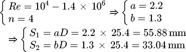
The set of pipes is specified by relative sloping step  , length step
  , and diameter step
  between axes of pipes. Based on the previous studies by researchers, from the viewpoint of heat transfer, the staggered arrangement is very effective. In this work, the values a and b are determined considering Reynolds number and the number of cylinders [16,17].
 These distances and steps have been used in arrangement of cylinders with respect to each other and in computational networking for experimental and theoretical works. The arrangement of cylinders is shown in Figure 1.
 |
Fig. 1 The arrangement of cylinders in the model. |
4.2 Numerical solution field and computational network
The numerical solution field used in this work is a 3-d field, which is shown in Figure 2. Considering Figure 2 and division values of field boundaries given below, the computational network is generated Table 5.
Figure 3 shows the computational network, the 486 elements, and the nodes.
It should be mentioned that in selecting the distance of the nodes, firstly the problem is solved for a large network, and then gradually the network is made smaller until the field dimensions of 0.635 × 0.4 × 0.4 is determined as an appropriate numerical solution field; and this field was used in numerical solutions. Also, different networking was applied on the model, and finally the determined network was used. This network satisfies the important condition that solutions and results must be independent of the network.
 |
Fig. 2 Numerical solution field. |
Divisions of computational network.
 |
Fig. 3 (a) Computational network, (b) elements of computational network, (c) nodes of computational network. |
4.3 Boundary conditions
Applying appropriate boundary conditions plays an important role in the process of numerical solution. Conditions in field input i.e. nozzle outlet are very important in the prediction of velocity in the center of jet and shear stresses. Velocity profile in the nozzle outlet is affected by the designing properties of nozzle such as proportion of length to diameter, shape of nozzle, possibility or impossibility of the presence of transfer region in upper-hand flow of nozzle. Here, the velocity profile in the nozzle outlet is assumed to be uniform [22–24] and the conditions of flow input in computation domain are stated as [25]:
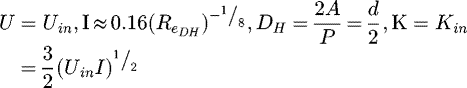 (39)
where
(39)
where  is Reynolds number based on hydraulic diameter, A is cross section and P is perimeter length. Table 6 gives the input conditions for the velocities between 100 m/s and 150 m/s. Therefore, boundary condition of input velocity is applied on the G surface.
Whereas a pressure equal to atmospheric pressure is applied to the surfaces A, B, C and D, therefore, the boundary condition applied to the surfaces A, C and D is defined as input pressure boundary condition and the boundary condition applied to the surface B is defined as output pressure boundary condition. These conditions are applied considering the real conditions of the test system. Also, taking into account the no-slip condition, the velocity on rigid surfaces such as the surface of cylinders and their holder walls, i.e. E and F, are considered as zero [26]. Therefore, wall boundary condition is defined for them.
Input conditions for the velocities between 100 and 150 m/s.
5 The stages of performing numerical analyses
The problem under study is analyzed in the following states (Fig. 4):
-
The nozzle is put in front of cylinder, and considering L = 1.52 D, the problem is analyzed in 3-d state for the values of Un equal to 100, 110, 120, 130, 140, 150 m/s.
-
The distance of nozzle outlet orifice from front edge of cylinder are assumed to be 1 D, 2 D and 3 D, respectively, and the problem is analyzed for the values of Un equal to 100 m/s (incompressible flow) and 150 m/s (compressible flow).
-
The jet (i.e. nozzle), in five steps and in each step to the amount of 0.2 of cylinder radius has been moved to the top, in a way that in the last step the axis of symmetry of the jet is tangential to the upper surface of the first cylinder. In this stage L = 1.52 D and Un = 100 m/s.
-
Like the third stage, the jet, in five steps and in each step to the amount of 0.2 of cylinder radius has been moved to the bottom, in a way that in the last step, the axis of symmetry of the jet is tangential to the lower surface of the first cylinder. In this stage L = 1.52 D and Un = 100 m/s.
-
Considering L = 1.52 D, and without eccentricity, besides RSM turbulence model (which was considered as turbulence model in all the above states), the problem is analyzed with the other three two-equation models as standard k-ε, RNG k-ε and realizable k-ε. In this state, Un is considered as 100 m/s.
6 Experimental model
The experimental model presented in Figure 5 is established to analyze the accuracy of the results obtained from the numerical solution. Before starting the experiments, the test platform must be located on a flat place, and be completely leveled. Also, connecting hoses related to nozzle and manometers must be controlled to completely establish the connections. After ensuring that the nozzle is placed in its place, the valve of air input from the compressor is opened, and considering the mounted outlets on the nozzle body, the velocity of the nozzle output flow is adjusted. The exit air flow from the nozzle encounters with the surface of the first cylinder and due to Coanda effect turns to the direction of other cylinders. After adjusting the height of nozzle and the main cylinder in different positions of the angle θ, corresponding pressure height in the boundary layer is measured.
The other side of the manometer is in contact with atmosphere.
 |
Fig. 4 Schematic of the cylinder in front of the jet and in different eccentricities. |
 |
Fig. 5 Schematic of the test system. 1, 2, 3, 4 – Circular cylinders that are capable of circulation around their axis of symmetry; 5, 6 – Walls with materials of Perspex glass, which are surrounded by wooden frames and have the duty to hold the cylinders; 7 – Nozzle; 8 – Fixed part of nozzle holder frame 9- Moving part of nozzle holder frame; 10, 11 – Regulating screws of nozzle height; 12 – Conveyer for adjusting the amount of circulation in circular cylinder; 13 – Index for determination of the amount of cylinder circulation; 14 – The main frame that all the above components are located on it; 15 – Screws for binding the cylinders to the walls of Perspex glass material with wooden frames. At the end of nozzle and cylinders, there are some parts that are shown in the Figures 6a and 6b and are defined as: (a) Location of connecting the pipe that is fed from air compressor and contains compressed; air. (b) Pressure outlet on the cylinder that is connected to a side of a U-shaped manometer to measure the pressure on the surface of cylinder. |
7 The stages of performing experimental analyses
Experimental tests have been performed in three stages. In all the stages, the distance between the nozzle outlet orifice and the front edge of the first cylinder, specified by L in Figure 4, has been chosen as 1.52 D. Also, in all the stages, the velocity of the exit air from the nozzle orifice has been chosen as 100 m/s. The stages of performing the test are as follows.
-
The nozzle is located exactly in front of the first cylinder. At this stage, there is no eccentricity and the pressure distribution on the surface of the first cylinder is measured and recorded, exactly in front of the jet. In order to measure the pressure, the first cylinder, in each part to the amount of 10 degrees, is circulated around its axis of symmetry. The process is repeated for the other cylinders. Therefore, in each testing, 4 × 36 numbers of information are required;
-
In the second stage, the jet (i.e. nozzle), in five steps and in each step to the amount of 0.2 of cylinder radius is moved to the top, in a way that in the last step the axis of symmetry of the jet is tangential to the upper surface of the first cylinder. In this stage, in each step, 4 × 36 numbers of information are recorded;
-
In the last stage of experimental tests, the nozzle, in five steps and in each step to the amount of 0.2 of cylinder radius is moved to the bottom, in a way that in the last step, the axis of symmetry of the jet is tangential to the lower surface of the first cylinder. In this stage, too, in each step, 4 × 36 numbers of information are recorded.
 |
Fig. 6 Nozzle. |
8 Presentation of results
Contours of velocity are shown in Figure 7 for the two states a) without eccentricity and L = 1.52 D, Un = 100 m/s and b) without eccentricity and L = 1.52 D, Un = 150 m/s, in yz plane. As it can be observed, the velocity of the flow from the output of nozzle to impinging point is decreased gradually in the central line of jet, which is close to zero in the resting point. At this point, the pressure reaches to its maximum value and also in the state without eccentricity the velocity profile has rather uniform distribution, which is begun from the value close to zero and is reached to a maximum value, and then is approached to the zero value again.
Also, in the eccentricity states, due to the Coanda effect, in spite of departing, the jet is pulled towards the cylinders, which is shown by Figures 8a and 8b.
In Figures 9 and 10, the procedures of shear stress distribution and pressure distribution, in 3-d, on the surface of first cylinder are shown, respectively. Also, in Figures 11 and 12, shear stress and pressure distributions, on the surface of first cylinder, along the axis of symmetry of jet, are presented, respectively. It should be mentioned that in all the figures, the shear stress and pressure have been non-dimensioned by velocity square of jet in nozzle outlet orifice and density. Pa is the pressure of atmosphere. It can be deduced from the figures that when the shear stress has the lowest value, the pressure has the highest value, because at these points velocity gradients have their minimum value. Also, it can be observed that in the angles with value about ±60∘, shear stress reaches to its maximum value.
In Figures 13a and 13b, a comparison has been shown between shear stresses on the first cylinder exactly in front of the jet, for various values of L between 1 D and 3 D, and for the values of Un as 100 m/s and 150 m/s, for the first cylinder. Results show that the distance of L = 1.52 D is an optimal distance for both the compressible and incompressible fluids, where the shear stress has its highest value on the surface of the first cylinder, i.e. in this state, the effect of the cleaning of the jet is higher than other states.
Figures 14a and 14b show the comparison between shear stress on the first cylinder and exactly in front of the jet for the states with different eccentricities between zero and 1R, where L = 1.52 D and Un = 100 m/s, and for the movement of the nozzle to the bottom or top, respectively. It can be observed that the shear stress, compared to other states, is the highest in the without eccentricity state. Also, considering the curves of the velocity level, it can be seen that applying eccentricity, the flow passing region moves to the back of the cylinder.
Figure 15 gives a comparison between shear stresses on the first cylinder exactly in front the jet for the output velocities between 100 m/s and 150 m/s. It can be observed that by increasing the velocity, the shear stress on the surface of the cylinder is increased, due to the increase in velocity gradients.
The presented experimental results for the velocity Un = 100 m/s and the state L = 1.52 D have been obtained with different eccentricities of the nozzle with respect to the first cylinder between zero and 1R, where some of the results have been compared to the numerical results in Figures 16a and 16b. Because of the limitations of the laboratory equipment for measuring the various properties of flow such as velocity in different regions, only the results obtained from measuring the pressure on the surface of cylinders are comparable with computer models.
In Figures 17a–Figure 17d, the results obtained from experimental analysis are compared to the results obtained from numerical solution applying different turbulence models, i.e. standard k-ε turbulence model, RSM turbulence model, RNG k-ε model and realizable k-ε model. The comparison shows that in the regions before separation point, all the models give predictions close to each other, and the difference appears after the separation point and in the flow passing region, where the comparison between numerical and experimental results shows that the RSM model has higher accuracy among all the models, however, its convergence speed is lower than other models, because in RSM model, more equations are solved. Also, results show that the standard k-ε model is weak in predicting the reverse and circulation flows, and the flow passing region.
In performing the tests and measuring the pressure some errors, such as error in adjusting the exit air velocity in the nozzle orifice, error in accurate adjusting of eccentricity, error in reading values and etc. occur that must not be neglected. Though, it is tried to lower the above errors as much as possible.
 |
Fig. 7 Velocity contour for numerical solution of field. |
 |
Fig. 8 Velocity contour for numerical solution of field; With eccentricity state, movement to top and bottom, L = 1.52 D, Un = 100 m/s, and Offset = 1R. |
 |
Fig. 9 The procedure of shear stress distribution on the surface of first cylinder (without eccentricity state; L = 1.52 D, Un=100 m/s). |
 |
Fig. 10 The procedure of pressure distribution on the surface of first cylinder (without eccentricity state; L = 1.52 D, Un = 100 m/s). |
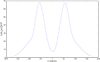 |
Fig. 11 Shear stress distribution on the surface of the first cylinder along the axis of symmetry of the jet. |
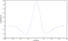 |
Fig. 12 Pressure distribution on the surface of the first cylinder along the axis of symmetry of the jet. |
 |
Fig. 13 Shear stresses on the first cylinder along the axis of symmetry of the jet; without eccentricity state and L = 1.52D. |
 |
Fig. 14 Shear stresses on the first cylinder along the axis of symmetry of the jet; without eccentricity state and L = 1.52D. |
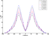 |
Fig. 15 Shear stresses on the first cylinder along the axis of symmetry of the jet. |
 |
Fig. 16 Comparison of non-dimensioned pressure distribution between the numerical and experimental solution methods on the first cylinder; L =1.52 D, Un=100 m/s. |
 |
Fig. 17 Comparison of non-dimensioned pressure distribution between numerical and experimental solutions on the first cylinder, applying different turbulence models; L = 1.52D, Un = 100 m/s, Offset = 0R. |
9 Conclusion
Considering the results obtained from the state of without eccentricity, it can be observed that for the optimal distance L = 1.52 D, in 3-d, the shear stress has its maximum value. In other words, in the stated distance, the jet has the highest cleaning effect, and by making nozzle distant from or close to the first cylinder, the shear stress becomes lower than the optimal state. This is true for both the states of incompressible fluid (Un =100 m/s) and compressible fluid (Un = 150 m/s).
The results show that when applying eccentricity to the first cylinder, in the state of without eccentricity the shear stress is lower than other states. Also, applying different eccentricities to the first cylinder, the separation point moves to the back of the cylinder and so the jet affects a large part of the first cylinder. In other words, the areas that were in the flow passing region and had not been cleaned, applying the eccentricity, went out of the flow passing region and were cleaned. The presence of other cylinders shrinks the domain of the flow passing region and causes a large part of the back of the cylinder to be cleaned.
As it is obvious from the results, for the first cylinder in a specified distance of nozzle to the first cylinder, increasing the output velocity of the nozzle causes the cleaning effect of jet on the surface of first cylinder to be increased. Because, increasing the nozzle output velocity, the shear stress and consequently the cleaning effect on the surface of the first cylinder increased.
Therefore, it can be stated that in order for cleaning the heat exchangers pipes, a fluid of jet (such as air jet) with high velocity can be used, so that it moves parallel with the diameter of the cylinder and sweeps the surface of the cylinder.
References
- S.H. Kang, R. Greif, Flow and heat transfer to a circular cylinder with hot impinging air jet, Int. J. Heat Mass Transfer 35 (1992) 2173–2183 [Google Scholar]
- S.P. Alavi Tabrizi, Turbulent Jet Impinging On Circular Cylinder, Ph.D Thesis, University Of Liverpool England, 1996 [Google Scholar]
- Imani Rad Reza, Study of two dimensional turbulent jet impinging on a cylinder at different eccentricities using various turbulence models, Ms Thesis, Faculty of Technical, Tabriz University, Iran, 1998 [Google Scholar]
- Motallebzade Rogayye, Study of two dimensional turbulent jet impinging on two cylinders, which was relative to the cylinder axis with a 45-degree angle, Ms Thesis, Faculty of Technical, Tabriz University, Iran, 1998 [Google Scholar]
- Javadi Khodayar, Numerical and experimental study of two dimensional turbulent jet impinging on two parallel cylinders, Ms. Thesis, Faculty of Technical, Tabriz University, Iran, 2000 [Google Scholar]
- Tahavor Alireza, Numerical and experimental study of a symmetric jet impinging on a cylinder in the direction of the perpendicular to the cylinder axis at the various eccentricities, Ms Thesis, Faculty of Technical, Tabriz University, Iran, 2001 [Google Scholar]
- B.E Launder, D.B. Spalding, The numerical computation of turbulent flows, Comput. Methods Appl. Mech. Eng. 3 (1974) 269–289 [Google Scholar]
- D.C. Wilcox, Turbulence modeling for CFD. DCW Industries, Inc., La Canada, California, 1993 [Google Scholar]
- B.E. Launder, D.B. Spalding, Lectures in mathematical models of turbulence, Academic Press, London, England, 1972 [Google Scholar]
- D. Choudhury, Introduction to the renormalization group method and turbulence modeling. fluent Inc. Technical Memorandum TM-107, 1993 [Google Scholar]
- T.H. Shih, W.W. Lieu, A. Shabbier, J. Zhu, A new k − ϵ Eddy-viscosity model for high Reynolds Number turbulent flows model department and validation, Comput. Fluids 24 (1995) 227–238 [CrossRef] [Google Scholar]
- S.E. Kim, D. Choudhury, B. Patel, Computations of complex turbulent flows using the commercial code fluent. in Proceedings of the ICASE/LaRC/AFOSR symposium on Modeling Complex Turbulent Flows, Hampton, Virginia, 1997 [Google Scholar]
- W.C. Reynolds, Fundamentals of turbulence for turbulence modeling and simulation. Lecture Notes for Von Kerman Institute Agard Report No. 755 1987 [Google Scholar]
- M.M. Gibson, B.E. Launder, Ground Effects on pressure fluctuations in the atmospheric boundary layer, J. Fluid Mech. 86 (1978) 491–511 [CrossRef] [Google Scholar]
- B.E. Launder, Second-moment closure: present… and future? Inter J. Heat Fluid Flow 10 (1989) 282–300 [CrossRef] [Google Scholar]
- B.E. Launder, G.J. Reece, W Rodi, Progress in The development of a Reynolds-Stress turbulence closure, J .Fluid Mech. 68 (1975) 537–566 [Google Scholar]
- B.J. Daly, F.H. Harlow, Transport equations in turbulence, Phys. Fluids 13 (1970) 2634–2649 [CrossRef] [Google Scholar]
- F.S. Lien, M.A. Leschziner, Assessment of turbulent transport models including non-linear rng eddy-viscosity formulation and second-moment closure Comput. Fluids 23 (1994) 983–1004 [Google Scholar]
- S. Fu, B.E. Launder, M.A. Leschziner, Modeling strongly swirling recirculating jet flow with Reynolds-Stress transport closures in sixth symposium on Turbulent Shear Flows, Toulouse, France, 1987 [Google Scholar]
- B.E. Launder, Second-moment closure and its use in modeling turbulent industrial flows, Int. J. Numer. Methods Fluids 9 (1989) 963–985 [CrossRef] [Google Scholar]
- S. Sarkar, L. Balakrishnan, Application of a Reynolds-Stress turbulence model to the compressible shear layer, ICASE Report 90-18, NASA CR 182002, 1990 [Google Scholar]
- S.E. Kim, D. Choudhury, A Near-Wall treatment using wall functions sensitized to pressure gradient, In ASME FED Vol. 217, Separated and Complex Flows, ASME., 1995 [Google Scholar]
- A. Zukauskas, R. Ulinskas Heat transfer in tube banks in cross flow, Springer- Verlag Berlin, 1988 [Google Scholar]
- I.H. Shames, Mechanics of Fluids, McGraw Hill Book Co., 1982, 281–282 [Google Scholar]
- B.E. Launder, D.B. Spalding, The numerical computation of turbulent flows, Comput. Methods Appl. Mech. Eng. 3 (1974) 269–289 [Google Scholar]
- S.H. Kang, R. Greif, Flow and heat transfer to a circular cylinder with hot impinging air jet, Int. J. Heat Mass Transf. 35 (1992) 2173–2183 [CrossRef] [Google Scholar]
Cite this article as: E. Jamalei, R. Alayi, A. Kasaeian, F. Kasaeian, M.H. Ahmadi, Numerical and experimental study of a jet impinging with axial symmetry with a set of heat exchanger tubes, Mechanics & Industry 19, 106 (2018)
All Tables
All Figures
|
Fig. 1 The arrangement of cylinders in the model. |
| In the text | |
|
Fig. 2 Numerical solution field. |
| In the text | |
|
Fig. 3 (a) Computational network, (b) elements of computational network, (c) nodes of computational network. |
| In the text | |
|
Fig. 4 Schematic of the cylinder in front of the jet and in different eccentricities. |
| In the text | |
|
Fig. 5 Schematic of the test system. 1, 2, 3, 4 – Circular cylinders that are capable of circulation around their axis of symmetry; 5, 6 – Walls with materials of Perspex glass, which are surrounded by wooden frames and have the duty to hold the cylinders; 7 – Nozzle; 8 – Fixed part of nozzle holder frame 9- Moving part of nozzle holder frame; 10, 11 – Regulating screws of nozzle height; 12 – Conveyer for adjusting the amount of circulation in circular cylinder; 13 – Index for determination of the amount of cylinder circulation; 14 – The main frame that all the above components are located on it; 15 – Screws for binding the cylinders to the walls of Perspex glass material with wooden frames. At the end of nozzle and cylinders, there are some parts that are shown in the Figures 6a and 6b and are defined as: (a) Location of connecting the pipe that is fed from air compressor and contains compressed; air. (b) Pressure outlet on the cylinder that is connected to a side of a U-shaped manometer to measure the pressure on the surface of cylinder. |
| In the text | |
|
Fig. 6 Nozzle. |
| In the text | |
|
Fig. 7 Velocity contour for numerical solution of field. |
| In the text | |
|
Fig. 8 Velocity contour for numerical solution of field; With eccentricity state, movement to top and bottom, L = 1.52 D, Un = 100 m/s, and Offset = 1R. |
| In the text | |
|
Fig. 9 The procedure of shear stress distribution on the surface of first cylinder (without eccentricity state; L = 1.52 D, Un=100 m/s). |
| In the text | |
|
Fig. 10 The procedure of pressure distribution on the surface of first cylinder (without eccentricity state; L = 1.52 D, Un = 100 m/s). |
| In the text | |
|
Fig. 11 Shear stress distribution on the surface of the first cylinder along the axis of symmetry of the jet. |
| In the text | |
|
Fig. 12 Pressure distribution on the surface of the first cylinder along the axis of symmetry of the jet. |
| In the text | |
|
Fig. 13 Shear stresses on the first cylinder along the axis of symmetry of the jet; without eccentricity state and L = 1.52D. |
| In the text | |
|
Fig. 14 Shear stresses on the first cylinder along the axis of symmetry of the jet; without eccentricity state and L = 1.52D. |
| In the text | |
|
Fig. 15 Shear stresses on the first cylinder along the axis of symmetry of the jet. |
| In the text | |
|
Fig. 16 Comparison of non-dimensioned pressure distribution between the numerical and experimental solution methods on the first cylinder; L =1.52 D, Un=100 m/s. |
| In the text | |
|
Fig. 17 Comparison of non-dimensioned pressure distribution between numerical and experimental solutions on the first cylinder, applying different turbulence models; L = 1.52D, Un = 100 m/s, Offset = 0R. |
| In the text | |
Current usage metrics show cumulative count of Article Views (full-text article views including HTML views, PDF and ePub downloads, according to the available data) and Abstracts Views on Vision4Press platform.
Data correspond to usage on the plateform after 2015. The current usage metrics is available 48-96 hours after online publication and is updated daily on week days.
Initial download of the metrics may take a while.