© N. Morin et al., Published by EDP Sciences, 2024

1 Introduction

Hydroelectric turbines are mechanical systems converting water flow energy to electricity. In a Francis turbine, the spiral casing creates a free water swirl (see Fig. 1). The runner transfers the water swirl's kinetic and potential energy in shaft torque by the transfer of momentum from the deflection of the water. By its function, the runner response is characterized by high dynamic stresses and its failure represents a costly loss of production [1]. The recent arrival of intermittent energy sources on the power grid stretches the operating range of those hydroelectric turbine-generator units. Off-peak operations of turbines result in new loadings accentuating fatigue degradation runners [2,3]. This new reality combined with the financial criticality of the integrity of the runner entails the need to comprehend its dynamic behaviour and loadings. This understanding should improve fatigue analysis, life estimation and diagnosis tools, and allow better-suited design of turbines to the fluctuating demand.

Typically, the modal characterization method for the runner is numerical simulations using an axisymmetric runner in a constrained acoustic fluid volume. Such a method usually considers isolated components like the runner with or without the shaft. Experimental methods are sometimes used to validate and calibrate numerical simulations [5–7]. Those experimental methods, however, consider the sole runner in air or standstill water ([5,8–10]) which is insufficient to capture the actual fluid-structure coupling effects found in operation. In essence, Operational Modal Analysis (OMA) methods use in situ measurements which account for the actual geometry of the runner and coupling and added mass effects. Such an identification approach is output-only assuming white noise excitation from the environment [11]. To account for uncertainty, Dollon et al. (2020) proposed a Bayesian modal analysis method using strain gauge measurements on runner blades in transient regimes [12]. However, in steady-state regimes near the Best Efficiency Point (BEP), periodic excitations dominate stochastic excitations, limiting the use of traditional OMA methods. Using runner strain measurements, Dollon et al. (2023) observed unexpected resonance between rotation speed harmonics and natural modes of the runner [4]. The author proposed a steady-state periodic forced response model to describe those Non-Trivial Runner-Casing interactions (NTRCI). The proposed model generalizes the Rotor-Stator Interactions (RSI) theory, which is the interaction of the rotating runner with the fixed Z_G guide vanes [13,14]. The identification of the periodic forced response model using strain gauge measurements presents an opportunity to achieve a harmonic-based modal analysis of the turbine runner, i.e., its harmonic modal analysis.

This paper presents a Bayesian inference method for the harmonic modal analysis of a Francis turbine runner using in situ strain gauge measurements. The paper is structured as follows. Section 2 presents the runner blades' periodic forced response model. Section 3 proposes an inference methodology to evaluate the runner's NTRCI excitation and modal parameters. Section 4 circumscribes the range of applicability of the algorithm through a synthetic data study. Section 5 presents the implementation of the method on an operational prototype runner under a NTRCI excitation. Section 6 discusses perspectives on future developments and applications of the method before concluding in Section 7.

Fig. 1 Principal components of Francis turbines from Dollon et al. (2023).

2 Periodic forced response model

Dollon et al. (2023) proposed a model to estimate the forced response of a runner blade to a purely periodic excitation by the analysis of one runner blade. The model states that, in the modal basis, the excitation generates Q harmonics per nodal diameter v, Q being a number depending on the considered bandwidth. The number of nodal diameters v is a quantity used to characterize the spatial shape of a mode of vibration in an axisymmetric structure [9,14]. Runner nodal diameters v are integers from $\left]-Z_{\text{R}}/2,Z_{\text{R}}/2\right[$ if the number of blades Z_R is odd or [(1 − Z_R)/2, (Z_R − 1)/2] if Z_R is even. The rotating runner's gyroscopic effect splits each stationary modes of a given nodal diameter v in two traveling waves ±v. In this paper, negative nodal diameters are counterrotating (backward) modes, and positive nodal diameters v (or ND) are corotating (forward) modes. Nodal diameter v = 0 is a standing vibration, considered as a backward mode in the model.

As described per Dollon et al. (2023), on an observed point n on the blade, the corotating angular position θ dependant shape F(θ) of the periodic excitation force in the physical basis can be expressed by a set of Fourier coefficients {F_p}. For a Z_R-bladed runner, the force projected in the modal basis, using a cardinal sine function, generates a harmonic excitation as expressed in equation (1) (q ∈ [1, Q]).

$$c_{q,v}={\displaystyle {{\displaystyle \sum }}_{p\in \mathbb{Z}}}{F}_p^{*}\text{sinc}\left[\left(q-p\right)\pi +\frac{\pi v}{Z_{\text{R}}}\right]e^{i\left[\left(q-p\right)\pi +\frac{\pi v}{Z_{\text{R}}}\right]}\approx F^{1\text{Z}}{\text{φ}}_{q,\nu }^{1\text{Z}}.$$(1)

In equation (1), c_q,ν ∈ ℂ^N×1 contains the excitation Fourier coefficients, F^1Z ∈ ℂ^N×(2P+1) contains a finite quantity P of force Fourier coefficients for a one-per-revolution force, N stands for the number of observations on a blade and ${\text{φ}}_{q,\nu }^{1Z}\in {ℂ}^{\left(2P+1\right)\times 1}$ is the transformation vector expressing the excitation force in the modal basis as illustrated in Figure 2. In Figure 2, on the left, are the Fourier coefficients {F_p} defining the one per blade per revolution (Z_R periodic) runner excitation expressed in Power Spectral Density as a function of multiples p of the harmonic orders of Z_R. On the right, the same excitation is expressed in the modal basis as a set of Z_R Q nodal diameter specific Fourier coefficients {c_q,v} in relation to the harmonic order of the runner rotation frequency Ω at an observed point n.

In the periodic response (see Eqs. (2) and (3)), an excitation harmonic's c_q,v magnitude is modulated according to its frequency proximity to corresponding natural frequencies ω_v,λ, with mode λ ∈ [1, Λ] of given normalized mode shape ψ_v,λ ∈ ℂ^N×1. The gyroscopic effect from rotation at frequency Ω causes each mode to split in conjugated forward (ω_+v,λ and ψ_+v,λ) and backward (ω_−v,λ and ψ_−v,λ) modes [4,15]. As developed in [4], the model deals with a single mode per nodal diameter. Here, the forced response model was adapted to a multimode λ contribution and expressed in the frequency domain in equations (2) and (3).

$$x_{q,+\nu }={\displaystyle {{\displaystyle \sum }}_{\lambda }}\frac{\sqrt{2\pi }}{{\omega }_{+\nu ,\lambda }-\left(q{Z}_R+\nu \right)\text{Ω}}{A}_{+\nu ,\lambda }{c}_{q,+\nu }\delta \left[f-\left(q{Z}_{\text{R}}+\nu \right)\text{Ω}\right]$$(2)

$$x_{q,-\nu }={\displaystyle {{\displaystyle \sum }}_{\lambda }}\frac{\sqrt{2\pi }}{-{\omega }_{-\nu ,\lambda }-\left(q{Z}_R-\nu \right)\text{Ω}}{A}_{-\nu ,\lambda }{c}_{q,-\nu }^{*}\delta \left[f-\left(q{Z}_{\text{R}}-\nu \right)\text{Ω}\right]$$(3)

In equations (2) and (3), x_q,v  ∈  ℂ^N×1 contains the q^th response harmonic for all observed points N on the blade, A_+v,λ A_−v,λ and A_−v,λ  Element of  ℂ^N×N are the residual matrices of the λ^th forward and backward conjugated modes of nodal diameter v, respectively. A residual matrix A_v,λ depends on normalized mode shape ψ_v,λ as $A_{\nu ,\lambda }={\psi }_{\nu ,\lambda }^{}{{\psi }_{v,\lambda }^H}^{}$. For a given excitation periodicity, equations (1), (2) and (3) can be combined in a matrix stacking all N × Q harmonics related to a given forward or backward nodal diameter ν as shown in equation (4):

$$X_{\nu }={\displaystyle {{\displaystyle \sum }}_{\lambda }}{A}_{\nu ,\lambda }F{\Phi }_{\nu }{W}_{\nu ,\lambda }$$(4)

where X_ν ∈ ℂ^N×Q contains the response harmonics, $F=\left[\begin{array}{ccc}\hfill F_0\hfill & \hfill F_{-p}\hfill & \hfill F_p\hfill \end{array}\right]\in {ℂ}^{N\times \left(2P+1\right)}$, with p ∈ [1, P], contains the excitation Fourier coefficients,${\text{Φ}}_{\nu }={\left[\begin{array}{ccc}\hfill {\text{φ}}_0\hfill & \hfill {\text{φ}}_{-p}\hfill & \hfill {\text{φ}}_p\hfill \end{array}\right]}^T\in {ℂ}^{\left(2P+1\right)\times Q}$ is the transformation matrix and W_ν,λ ∈ ℝ^Q×Q is a diagonal matrix with element $W_{qq}=\frac{\sqrt{2\pi }}{{\omega }_{+\nu ,\lambda }-\left(q{Z}_R+\nu \right)\text{Ω}}$ or $\frac{\sqrt{2\pi }}{-{\omega }_{-\nu ,\lambda }-\left(q{Z}_R-\nu \right)\text{Ω}}$ for forward or backward modes.

Francis turbines' excitation inevitably contains rotor-stator interactions (RSI), which are Z_G-periodic forces. To obtain an excitation model accounting for RSI, a Z_G periodic excitation is added to the initial 1Z excited model as: $X_{\nu }^{1Z,Z_{\text{G}}Z}={\displaystyle {{\displaystyle \sum }}_{\lambda }}{A}_{\nu ,\lambda }{F}^{1Z,Z_{\text{G}}Z}{\text{φ}}_{\nu }^{1Z,Z_{\text{G}}Z}{W}_{\nu ,\lambda }$, where $X_{\nu }^{1Z,Z_{G}Z}\in {ℂ}^{N\times Q}$ is the strain response matrix, $F^{1Z,Z_{\text{G}}Z}=\left[\begin{array}{cc}\hfill F^{1Z}\hfill & \hfill F^{Z_{G}Z}\hfill \end{array}\right]\in {ℂ}^{N\times 2\left(2P+1\right)}$and ${\text{φ}}_{\nu }^{1Z,Z_{\text{G}}Z}={\left[\begin{array}{cc}\hfill {\text{φ}}_{\nu }^{1Z}\hfill & \hfill {\text{φ}}_{\nu }^{Z_{\text{G}}Z}\hfill \end{array}\right]}^T\in {ℂ}^{2\left(2P+1\right)\times Q}$ are respectively the combined 1Z and RSI force coefficients and modal transformation matrices. To infer the excitation coefficients F of a given excitation, the mode shapes ψ_v,λ and natural frequencies ω^ν_λ, the ncontribution of a specific excitatioon the harmonics is isolated so that $X_{\nu }=X_{\nu }^{1Z,Z_{\text{G}}Z}-X_{\nu }^{\overline{Z}}$.

Fig. 2 Transformation of the excitation from the physical to the modal basis.

3 Model-based inference algorithm

The method used to fit the model to the measured strains synchronous harmonics of the runner is based on the Prediction Error Method (PEM) (Eq. (5)) [16]. The error ε between the measured harmonics ${\hat{X}}_{\nu }\in {ℂ}^{N\times Q}$ and the model X_ν is proposed complex Gaussian $\epsilon \sim N_C\left(0,{\sigma }^2{I}_{2NQ{Z}_{\text{R}}}\right)$ with σ² the variance of error ε.

$${\hat{X}}_{\nu }=X_{\nu }+\epsilon .$$(5)

Using Bayes' Theorem [17] with a uniform prior, the posterior density of probability of the model given the data, $𝒫\left(X_{\nu },{\sigma }^2|{\hat{X}}_{\nu }\right)$, is expressed proportional to the likelihood $L\left({\hat{X}}_{\nu }|X_{\nu },{\sigma }^2\right)$ of the data: $𝒫\left(X_{\nu },{\sigma }^2|{\hat{X}}_{\nu }\right)\propto L\left({\hat{X}}_{\nu }|X_{\nu },{\sigma }^2\right)$. The resulting complex Gaussian likelihood is expressed in equation (6).

$$L\left({\hat{X}}_{\nu }|X_{\nu },{\sigma }^2\right)\frac{1}{{\sigma }^{2NQ}}{e}^{-\frac{1}{{\sigma }^2}tr\left[{\left({\hat{X}}_{\nu }-X_{\nu }\right)}^H\left({\hat{X}}_{\nu }-X_{\nu }\right)\right]}$$(6)

From the likelihood, a conditional probability density is derived in Sections 3.1–3.3 for the error, the excitation and mode shapes enabling Gibbs sampling [17]. Since the conditional probability density shape of the natural frequencies is unknown, as shown in Section 3.4, a Metropolis-Hastings step is implemented leading to a Metropolis-Within-Gibbs algorithm [18].

3.1 Error sampling Kernel

The error depends on all response harmonics of the N observed points. Therefore, the conditional probability density is the product of every nodal diameter probability density. The obtained conditional probability density for the homoscedastic variance σ² is an inverse gamma distribution 𝒢⁻¹ as shown in equation (7).

$$p\left({\sigma }^2|\text{rest}\right)g^{-1}\left({\displaystyle \sum }_{\nu }2NQ-1,\hspace{0.17em}{\displaystyle \sum }_{\nu }\Vert {\hat{X}}_{\nu }-X_{\nu }{\Vert }^2\right)$$(7)

with rest being all the other parameters.

3.2 Excitation sampling Kernel

The excitation associated to an observed point n depends on each of its response harmonics. Using equation (6) and the model (Eq. (4)) as a vector $\text{vec}\left([\begin{array}{cc}\text{Re}\left(X_{\nu }\right)\hfill & \text{Im}\left(X_{\nu }\right){]}^T\hfill \end{array}\right)={\tilde{P}}_{\nu }\text{vec}\left(\tilde{F}\right)$, equation (8) expresses the conditional probability of the excitation, p (F|rest).

$$p\left(F\text{|rest}\right)\hspace{0.17em}\propto 𝒩\left({\displaystyle {\sum }_{\nu }}{\left({{\tilde{P}}_{\nu }}^T{\tilde{P}}_{\nu }\right)}^{-1}{{\tilde{P}}_{\nu }}^T\text{v}\text{e}\text{c}\left({\left[\begin{array}{cc}\hfill \text{Re}\left({\hat{X}}_{\nu }\right)\hfill & \hfill \text{Im}\left({\hat{X}}_{\nu }\right)\hfill \end{array}\right]}^T\right),{\sigma }^2{\displaystyle \sum }_{\nu }{\left({{\tilde{P}}_{\nu }}^T{\tilde{P}}_{\nu }\right)}^{-1}\hspace{0.17em}\right)$$(8)

with transformation matrix ${\tilde{P}}_{\nu }={\left[\begin{array}{cc}\hfill \text{Re}\left({\displaystyle \sum }_{\lambda }{W}_{\nu \lambda }{}^T{{\Phi }_{\nu }}^T\otimes A_{\nu \lambda }\right)\hfill & \hfill \text{Im}\left({\displaystyle \sum }_{\lambda }{W_{\nu \lambda }}^T{{\Phi }_{\nu }}^T\otimes A_{\nu \lambda }\right)\hfill \end{array}\right]}^T\in R^{2NQ\times 2N\left(2P+1\right)}$, the Kronecker product ⊗, and with $\tilde{F}=\left[\begin{array}{cc}\hfill \text{Re}\left(\left[\begin{array}{cc}\hfill F_0\hfill & \hfill F_p\hfill \end{array}\right]\right)\hfill & \hfill \text{Im}\left(F_p\right)\hfill \end{array}\right]\in {ℝ}^{N\times \left(2P+1\right)}$ being the excitation coefficients matrix expressed in the real space.

3.3 Mode shape sampling Kernel

Mode shapes are normalized complex vectors. Each mode λ has an associated mode shape. The conditional probability density for a given mode shape ψ_v,λ is evaluated with measured harmonics X̂_ν,λ considering the contribution of other modes as described in equation (9).

$${\hat{X}}_{\nu ,\lambda }={\hat{X}}_{\nu }-{\displaystyle \sum }_{\zeta \ne \lambda }{A}_{\nu ,\zeta }\hspace{0.17em}F\hspace{0.17em}{\Phi }_{\nu }{W}_{\nu ,\zeta }.$$(9)

From the proposed likelihood (Eq. (6)), mode shape vectors contained in residual matrices $A_{\nu ,\lambda }={\psi }_{\nu ,\lambda }{{\psi }_{\nu ,\lambda }}^H$ are factorized in equation (10) using the cyclic shift invariance of the trace.

$$L\left({\hat{X}}_{\nu ,\lambda }|X_{\nu ,\lambda \hspace{0.17em}},{\sigma }^2\right)\hspace{0.17em}{e}^{\text{t}\text{r}\left[{{\psi }_{\nu ,\lambda }}^H\left(\frac{-1}{{\sigma }^2}\left[F{\Phi }_{\nu ,\lambda }{W}_{\nu ,\lambda }{W_{\nu ,\lambda }}^T{{\Phi }_{\nu ,\lambda }}^H{F}^H-{\hat{X}}_{\nu ,\lambda }{W_{\nu ,\lambda }}^H{{\Phi }_{\nu ,\lambda }}^H{F_p}^H-F{\Phi }_{\nu ,\lambda }{W}_{\nu ,\lambda }{{\hat{X}}_{\nu ,\lambda }}^H\right]\right){\psi }_{\nu ,\lambda }\right]}.$$(10)

From equation (10), using Hoff (2009) developments, a vector Bingham conditional probability can be derived for a vector in ℂ^N×1, hence the normalized complex mode shape ψ_v,λ.

3.4 Natural frequency sampling Kernel

From the likelihood $L\left({\hat{X}}_{\nu ,\lambda }|X_{\nu ,\lambda },{\sigma }^2\right)$ (see Eq. (10)), the natural frequency ω_v,λ in the diagonal of W_v,λ has an intractable kernel shape. In a random walk Metropolis-Hastings step [17], candidates ω_v,λi at iteration i are sampled in a Gaussian distribution $({\omega }_{{v,\lambda }_{i-1}},{{\sigma }_{\lambda }}^2)$ with a user-defined variance ${{\sigma }_{\lambda }}^2$. To maximise the acceptance ratio of a given natural frequency ω_v,λ, variance ${{\sigma }_{\lambda }}^2$ can be defined natural frequency specific considering the signal-to-noise ratio (SNR) of given harmonics. In our case, as the rotating runner is expected to be excited from a point of the fixed domain, forward modes have lower SNR because they are excited by higher order harmonics than backward modes. Therefore, the inference of forward natural frequencies is more sensitive to stochastic excitation bias (see Sect. 4.1.3).

A hypothesis is made on mode-split from the gyroscopic effect, stating that the frequency gap between conjugate modes is in the range of 0 Hz to 10 Hz. A forward natural frequency density of probability p(ω_+v,λ |rest) is then weighted by a Gaussian prior p (ω_+ν,λ|ω_+ν,λ) = − (ω_+ν,λ − ω_−ν,λ)²/2k² given the backward natural frequency value ω_−v,λ and a user-defined variance k² influencing the natural frequency ω_v,λ samples.

$$p\left({\omega }_{+\nu ,\lambda }|\text{rest}\right)L\left({\hat{X}}_{\nu }|X_{\nu },\text{Σ\hspace{0.17em}}\right)p\left({\omega }_{+\nu ,\lambda }|{\omega }_{-\nu ,\lambda }\right).$$(11)

In the Metropolis-Hastings step of the algorithm, user-defined variances ${{\sigma }_{\lambda }}^2$ are tuned according to the noise level and the quantity N of observed points (sensors) considered for the inference to maximize the acceptance ratio of each natural frequency.

Many vibration modes can be associated with a given nodal diameter ± ν, e.g., a type of mode shape. The sampling of each nodal diameter-specific natural frequencies is executed sequentially. To ensure stability in the sampling, the order of those natural frequencies is constrained from the lower frequency mode to the higher frequency mode so that ω_ν,λ < ω_ν,λ+1.

4 Synthetic data study

The probabilistic modal identification algorithm is intended to be deployed on in situ measurements. It, therefore, needs to be evaluated on a representative synthetic dataset. Three groups of parameters interreact: the excitation periodicities, the number of harmonics accessible from the measured response and the number of modes contained in the analyzed frequency band.

4.1 Range of applicability

The measured synchronous harmonics in the studied datasets are observed up to around the 40th to 50th harmonic. In this frequency band, for our studied Francis runner, 3 to 7 modes λ per nodal diameter ν are expected. In this sense, as the harmonic order considered by the algorithm increases, so does the complexity of the forced response model to infer.

4.1.1 Minimal quantity of harmonics

Let's consider a system with two modes per nodal diameter, excited by a periodic force composed of a fundamental and three harmonics. This system is solved with five observed points n on one runner blade. From the experimentation results, the minimal number of harmonics required for Markov Chain Monte-Carlo (MCMC) convergence is Z_RQ = 39 for a Z_R= 13 blades runner, e.g., Q = 3 response harmonics per nodal diameter ν. When the periodic force is described by more (Q > 3) harmonics in the spectral domain, the MCMC stability for the excitation decreases. This observation is also made when the number of observed points n increases. However, this stability loss can be solved by adding higher-order response harmonics.

From the two mentioned limitations, the inference of a 2Z pattern or higher periodicity excitation, like RSI, from the Z_RQ ∼ 50 observable response harmonics in the response is unattainable. The one or two RSI-specific excitation harmonics observable can be ignored if still three harmonics per ND can be used for the inference. RSI excitation's amplitude contribution to 1Z-affected harmonics can be considered using a pseudo-inverse function to infer a residual amplitude for the RSI contribution to the harmonics.

4.1.2 Minimal quantity of modes

When the algorithm is tested on systems containing more than two modes per nodal diameter (ND), it causes a divergence in the excitation sampling. For a given nodal diameter ν, the modal residue induced by higher frequency modes introduces some inaccuracies in the inference, leading to a bias in the inference of the highest natural frequency, from now on called 2nd mode. The lowest natural frequency, e.g., first mode, is less altered suggesting that the higher frequency acts as a firewall that captures the higher frequency modes bias. A test was carried out where the algorithm tried to characterize two modes per ND from a synthetic signal generated using four modes per ND. Figure 3 illustrates the bias obtained for mode ND5-2 (2nd mode of the 5th nodal diameter). Without a frequency maximum constraint, some Markov Chains of the natural frequencies were also observed to drift towards higher frequencies in a multimodal shape.

To minimise the modal residue effect, forward and backward 2nd mode natural frequencies ND2-2 to ND6-2 are sampled using an independent Metropolis-Hastings method [17] based on a Gaussian distribution $\left({\omega }_{{\pm \nu ,2}_{\text{I}\text{W}}},{\sigma }_{\lambda }{2}^{}\right)$ with a constant defined mean ω_±ν,2 IW near the expected 2nd mode natural frequency and a variance ${\sigma }_{\lambda }{2}^{}=100$. A Gaussian prior g (ω_ν,λ|ω_−ν,λ) given the conjugate mode, and as initially defined for forward modes (Sect. 3.4), is also added on all 2nd modes sampling. The additions constrain the 2nd modes sampling around the expected 2nd mode natural frequency value to minimize the modal under-definition bias.

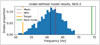Fig. 3 Algorithm mode under-definition bias effect on 2nd modes.

4.1.3 Stochastic excitation bias

On Francis turbine runners around the best efficiency point, stochastic excitations, dominated by periodic excitations, are marginal but non-zero. As the modelled excitation is proposed as purely periodic, the stochastic excitation contribution biases the model. The noise floor of strain measurements on an operating runner was analyzed at 70%, 50% and 20% of guide vanes opening (GVO) to evaluate the stochastic excitation level at each opening. For the analysis, the measured stochastic contribution to the signal at the three guide vanes openings is normalized using the noise floor level |2γ|² near the first harmonic order in the power spectrum and the power of the first synchronous harmonic |A₁|² as log [|2γ|²/|A₁|²]. Noise floor levels in the range of 20 GVO to 70 GVO were observed between log [|2γ|²/|A₁|²] = − 7.5 and log [|2γ|²/|A₁|²] = − 9.2, hence a lower stochastic contribution near the BEP.

The algorithm's sensitivity to the stochastic bias was evaluated using added Gaussian stochasticity to the excitation generating a harmonic to stochastic ratio (HSR) log [|2γ|²/|A₁|²] near the one measured at the tested GVO. The resulting absolute amplitude error for excitation parameters is of order 10⁻²N·s to 10⁻¹N·s for Gaussian stochastic contributions considered equivalent to 20 GVO and 70 GVO conditions. As the amplitude of the periodic excitation's Fourier coefficients increases, the bias becomes negligible. The stochastic bias sensitivity analysis showed that the proposed Gaussian stochastic excitation has no critical effect on the excitation parameters around BEP, e.g., log [2γ/|A₁|²] ≈ − 9, although the bias should be considered for better accuracy.

In the preceding analysis, the interaction between the stochastic excitation and the system was not considered. The resonance between the runner's vibration modes and the stochastic excitation could generate a non-negligible bias on the synchronous harmonics and should be investigated.

4.2 Synthetic data study case

The algorithm is evaluated using the 3Z_R first harmonics produced by a four modes per ND, model under a combined 1Z and RSI excitation observed by 10 sensors. The forces Fourier coefficients are defined using uniform distributions 𝒰. The fundamentals distributions are F_0,1Z = 𝒰 [85, 115] Y N · s and F_0,RSI = 𝒰 [985, 1015] Y N · s, with binary variable Y = ±1 with equal probability. The harmonics distributions are defined as F_p,1Z = 𝒰 [− 80, 80] and F_p,RSI = 𝒰 [− 710, 710]. Turbine parameters are Z_G=24 guide vanes, Z_R=13 runner blades and a Ω=1.25 Hz rotating frequency. The observed RSI harmonic is considered using a pseudo-inverse function. To simulate a 70% guide vane's opening with a non-negligible stochastic contribution to the periodic excitation based on Section 4.1.3 analysis, a Gaussian noise is added generating a HSR log [|2γ|²/|A₁|²] = − 8.13. Mode shapes are randomly generated, and natural frequencies are chosen in an actual runner-like range (see Tab. 1) based on previous modal analysis of the studied runner using finite element analysis in standstill water. In Figure 4, excitation harmonics generated by coefficients c_q,v are represented in red. Each harmonic's amplitude varies according to its proximity to the nodal diameter and companion-specific modes resulting in the strain response X_v in black. Forward modes harmonics are indicated by the minus sign. For visualization, the noise floor is represented among the harmonics. The probabilistic algorithm is set to infer the two firsts of the defined four modes per ND and three of the five defined excitation harmonics to reproduce an under-definition of the system as may occur on field measurements deployment.

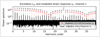Fig. 4 Excitation harmonics (red) modulated in the strain response (black).

4.3 Results on synthetic data

The model inference results over 60,000 iterations are shown in Table 1. The Most Probable Value (MPV) per natural frequency is compared to the defined target value by a relative error in percentage.

The Metropolis-Hasting candidate distribution for forward and backward modes ND2-2 to ND6-2 was set to a mean ω_±ν,2IW = 50Hz and variance ${{\sigma }_{\lambda }}^2=100$ for the inference.

In Table 1, torsion modes (ND0) harmonics have poor signal-to-noise ratio (SNR) and lead to inconclusive results. The obtained 95% credibility intervals (IC-95) for 1st modes vary from 1.5 Hz to 26.9 Hz. Also linked to low SNR harmonics, forward modes ND1^*-1 to ND6^*-1 are inferred with a 10 Hz to 20 Hz larger IC-95 than backward modes. The resulting IC-95 for 2nd modes, inferred with the independent candidate method, is in the range of 7.0 Hz à 24.6 Hz. Although the inferred 2nd modes may be biased, their consideration facilitates the inference of first modes as ND1-1 to ND6-1 are inferred within a 3 Hz error. The error over 14% for mode ND4-1 results from a bimodal posterior distribution for the parameter. The first mode (MPV-1) is found near 23 Hz and the second mode (MPV-2) is found near 27 Hz. Such a case shows that the analysis of the shape of the posterior distribution is necessary. The same analysis using 5 sensors showed similar results. Finally, the defined 2% to 10% mode split is within the error range.

5 Implementation on field measurements

The synthetic and the field measurements differ in the stochastic excitation influence and damping effects, among other epistemic uncertainties. To begin with, the stochastic excitation bias added to the model produces a constant broadband noise floor. In operation, turbulence excitation, cavitation and vortices might induce colored noise with an irregular floor interacting with the vibration modes of the system. The biased harmonics might be interpreted of higher amplitude than expected by the model, increasing risks of excitation overshooting or indetermination. Furthermore, damping is not accounted for in the model. This omission might lead to phase biases of the inferred excitation and mode shapes, and to an overestimation of synchronous harmonics amplitude for a given natural frequency. The algorithm is deployed on field measurements to evaluate the impact of the biases.

5.1 Field steady-state strain measurements

The studied runner is a low-head Francis turbine with Z_R= 13 blades, Z_G= 24 vanes and a rotating speed of Ω = 1.25 Hz. The strain and pressure measured points are shown in Figure 4.

The pressure measurements are used to analyze the possible excitation periodicities in the runner. As shown in Figure 5a, a dominant 1-per-revolution synchronous pressure amplitude is present in the system leading to the consideration that there is a 1Z excitation of the runner.

The rotating speed of the runner is not perfectly constant. Some runners' rotating speed respond to the grid power variations or are oscillating around a speed command. The synchronous vibrations are therefore extracted by synchronous averaging [20]. In Figure 6b, in green, are the extracted harmonic values from the runner strain response (black) measured by one of the strain gauges on the runner blade installed as shown in red in Figure 5. The extracted harmonics (green) are used for the inference of the model by the algorithm.

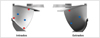Fig. 5 Strain (red) and pressure (blue) measured points.

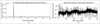Fig. 6 (a) 30°cm from leading edge intrados pressure measurements on blade 2. (b) Extracted harmonics (green) from the runner strain response (black) measured by one of the strain gauges on the runner blade.

5.2 Results on field measurements

The excitation, mode shapes and natural frequencies inference is completed with measurements from 10 strain gauges on two blades of the same runner during stable operation near the best efficiency point. The algorithm is set to infer, over 200k iterations, 26 modes and a one-per-revolution (1Z) excitation, considering the RSI response harmonic, defined with one fundamental and three harmonics. The first 15 of the 26 inferred modes' natural frequencies of the runner are presented in Table 2. The inferred natural frequencies are compared to numerical simulation results of the studied runner in standstill water. As the numerical simulation did not include the runner shaft, simulated ND1 natural frequencies are not considered.

From Table 2, the posterior distributions of forward modes natural frequencies ND2^*-1 to ND6^*-1 show similar IC-95, of 17.7 Hz to 23.1 Hz than the resulting distributions of the same modes with synthetic data. The MPV of natural frequencies obtained on field measurements are all within their IC-95 except for mode ND3-1 (22.1 Hz) which is only within its IC-99. The IC-95 obtained with blade 1 and 2 show a ±4 Hz consistency excepted for modes ND2-1 and ND2^*-1. The IC-95 of those inferred natural frequencies is 5.0 Hz to 7.0 Hz higher on blade 2 than on blade 1.

The MCMC of the excitation parameters showed partial stabilization. The reconstruction of the signal harmonics with the inferred model shows an up to 10⁴ µε overshoot of the harmonics over the 13th order and IC-95 on the excitation parameters of order 10³ N s.

On different tries with given measurements, a phase variability between the excitation Fourier coefficients and an up to 10 Hz variability of the inferred natural frequencies MPV were observed. As for the obtained IC-95 they vary by ±5 Hz. The blade difference of the MPV presented in Table 2 may therefore not only be attributed to the local physical properties of the two blades but to the variability of the different tries and the indetermination of the excitation with the actual model and data.

The omission of stochastic contribution to the system and damping may be the root cause of the non-repeatability and the partial stabilization of the excitation entailing the consideration necessity of those effects. As the proposed model is shown non-exhaustive for the used measurements, the inferred modal parameters may not be statistically conclusive.

6 Discussion and perspectives

The previous sections showed the inference of a periodic forced response model from synthetic data and operating runner strain measurements using a Bayesian inference-based algorithm. The complexity of the proposed model and method is noteworthy. Improperly constructed model matrices may lead to algorithm convergence but produce unphysical results. Therefore, validating the model and initially evaluating the algorithm on synthetic data are crucial to ensure satisfying results. Although the inferred natural frequency values in Section 5 are within the range of simulated natural frequencies, the method would benefit from future works to enhance the stability and resulting 95% credible intervals. Biases from stochastic excitations, modal residues and damping effects should be considered by the method. At first, stochastic excitations' contribution should be considered in the analysis as synchronous harmonics' amplitude might contain a non-negligible stochastic contribution that may cause the frequency-varying noise floor observed in the strain response (see Fig. 5b). If the noise floor variations are mainly random, Discrete Random Separation (DRS) [21] could be used. Other noise floor models or the combination of the proposed deterministic harmonic modal analysis method and stochastic excitation-based traditional OMA could be of interest. This consideration could enhance the accuracy and range of applicability of the method in different turbine operating regimes. Secondly, modal residue parameters should be added to the model as the algorithm is limited to the consideration of 2 modes per nodal diameter ν. The consideration could lead to a better accuracy in the 2nd modes inference. Then, as damping may be difficult to include as a parameter in the probabilistic algorithm, sensitivity analysis or model selection methods using proposed damping constants added to the model could be of interest. The exploitation of a numerical simulation of the studied runner could also be of interest. The simulated natural frequencies could be used as constants in the algorithm to estimate damping coefficients in the Metropolis-hastings step. As 2nd modes per nodal diameter may be more damped [8] the consideration of damping could correct the overshoot of the excitation and response harmonics by the algorithm.

A more exhaustive forced response model combined with the better-suited algorithm could not only become a useful tool for operating runner's dynamics characterization but also represent a harmonic modal analysis opportunity on model scale runners. On model-scale test benches, it may be possible to generate a controlled 1Z excitation by moving a specific guide vane. With mechanical homology principles [22], the natural frequencies of operating runners could be deducted. This less expensive and more flexible application of the method could lead to new knowledge on runners' dynamics and loadings.

7 Conclusion

In operating hydro-turbines, Non-Trivial Runner-Casing Interactions (NTRCI) can produce a wide range of synchronous harmonics observable in strain gauge measurements of the runner's response. Dollon et al. (2023) proposed a periodic forced response model, considering gyroscopic effects, explaining the nodal diameter specificity and amplitude of the harmonics. In this paper, a Bayesian method is proposed to infer the roots of a periodic excitation, modal characteristics, and uncertainties of Dollon et al. (2023) NTRCI model from observed harmonics in a Francis runner steady-sate strain response. The proposed method is limited to a case study under a one-per-revolution (1Z −NTRCI) and Rotor-Stator Interaction (RSI) combined excitation with dominant influence from the first 2 modes of each specific nodal diameter. The proposed algorithm inferred 15 of the first modes of an operating Francis runner within a 7.5 Hz difference of simulated natural frequencies in standstill water and a 95% credible interval (IC-95) of 8.0 Hz to 23.9 Hz. The considered rotating frequency-dependent mode split effect was shown insignificant compared to the quantified uncertainties. The partial stabilization and non-repeatability of the excitation inference imply the non-negligibility of stochastic excitations, modal residues and damping effects.

Future works focussing on improving stochastic excitation, modal residue and damping modelling could bring a more representative physical model. The Bayesian inference algorithm could benefit from combined blade information in the statistical model and mode coupling information. Parameter discrimination could be enhanced by using model selection methods and prior information from numerical simulations as Bayesian algorithms are well suited for the addition of prior knowledge. Ultimately, this harmonic modal analysis method could bring more knowledge on runners' dynamics and loadings, essential for design, life analysis tools and health monitoring.

Acknowledgements

I would like to express my gratitude to the scholar partners, ÉTS and Lab. Vibration Acoustique, and industrial partners, Andritz Hydro Canada Inc, Institut de Recherche d'Hydro-Québec (IREQ) and Mitacs, for their support of the project. The highly skilled and rigorous contributors on the partners' team, including Quentin Dollon, Jérôme Antoni, Antoine Tahan, Christine Monette and Martin Gagnon, played a crucial in the success of this research.

Funding

The Article Processing Charges for this article are taken in charge by the French Association of Mechanics (AFM).

Conflicts of interest

This research was performed as part of a Mitacs Accelerate program (https://www.mitacs.ca/our-programs/accelerate-core-business/) during Nicolas Morin's master's study program at l'École de Technologie Supérieure. As part of the program, Nicolas Morin received funding from Mitacs, Andritz, and Hydro-Québec.

Data availability

The authors do not have permission to share data.

Authorship contribution

N. Morin: Conceptualization, Methodology, Data curation, Writing − original draft. Q. Dollon: Reviewing and editing. J. Antoni: Reviewing and editing. A. Tahan: Reviewing and editing. C. Monette: Reviewing and editing. M. Gagnon: Reviewing and editing.

References

All Tables

All Figures

	Fig. 1 Principal components of Francis turbines from Dollon et al. (2023).
In the text

	Fig. 2 Transformation of the excitation from the physical to the modal basis.
In the text

	Fig. 3 Algorithm mode under-definition bias effect on 2nd modes.
In the text

	Fig. 4 Excitation harmonics (red) modulated in the strain response (black).
In the text

	Fig. 5 Strain (red) and pressure (blue) measured points.
In the text

	Fig. 6 (a) 30°cm from leading edge intrados pressure measurements on blade 2. (b) Extracted harmonics (green) from the runner strain response (black) measured by one of the strain gauges on the runner blade.
In the text

References

- X. Liu, Y. Luo, B.W. Karney, W. Wang, A selected literature review of efficiency improvements in hydraulic turbines, Renew. Sustain. Energy Rev. 51, 18–28 (2015) [CrossRef] [Google Scholar]
- C. Monette, H. Marmont, J. Chamberland-Lauzon, A. Skagerstrand, A. Coutu, J. Carlevi, Cost of enlarged operating zone for an existing Francis runner, IOP Conf. Ser.: Earth Environ. Sci. 49, 072018 (2016) [CrossRef] [Google Scholar]
- O. Savin, J. Baroth, C. Badina, S. Charbonnier, C. Bérenguer, Damage due to start-stop cycles of turbine runners under high-cycle fatigue, Int. J. Fatigue 153, 106458 (2021) [CrossRef] [Google Scholar]
- Q. Dollon, A. Tahan, J. Antoni, M. Gagnon, C. Monette, Toward a better understanding of synchronous vibrations in hydroelectric turbines, J. Sound Vibrat. 544, 117372 (2023) [CrossRef] [Google Scholar]
- T. Châteauvert, A. Tessier, Y. St-Amant, J. Nicolle, S. Houde, Parametric study and preliminary transposition of the modal and structural responses of the Tr-FRANCIS turbine at speed-no-load operating condition, J. Fluids Struct. 106, 103382 (2021) [CrossRef] [Google Scholar]
- M. Gagnon, Q. Dollon, J. Nicolle, J.-F. Morissette, Operational modal analysis of Francis turbine runner blades using transient measurements, IOP Conf. Ser.: Earth Environ. Sci. 774, 012082 (2021) [CrossRef] [Google Scholar]
- S. Lais, Q. Liang, U. Henggeler, T. Weiss, X. Escaler, E. Egusquiza, Dynamic analysis of francis runners − experiment and numerical simulation, Int. J. Fluid Mach. Syst. 2, 303–314 (2009) [CrossRef] [Google Scholar]
- D. Valentín, A. Presas, C. Valero, M. Egusquiza, E. Jou, E. Egusquiza, Influence of the hydrodynamic damping on the dynamic response of francis turbine runners, J. Fluids Struct. 90, 71–89 (2019) [CrossRef] [Google Scholar]
- D. Valentin, A. Presas, M. Bossio, E.M. Montagut, E. Egusquiza, C. Valero, Feasibility of detecting natural frequencies of hydraulic turbines while in operation, using strain gauges, Sensors 18, 174 (2018) [CrossRef] [PubMed] [Google Scholar]
- B. Graf, L. Chen, Correlation of Acoustic Fluid-Structural Interaction Method for Modal Analysis with Experimental Results of a Hydraulic Prototype Turbine Runner in Water. In international conference on noise and vibration, ISMA (2010), pp. 2489–2503 [Google Scholar]
- R. Brincker, C. Ventura, Introduction to operational modal analysis. John Wiley & Sons (2015) [Google Scholar]
- Q. Dollon, J. Antoni, A. Tahan, M. Gagnon, C. Monette, C. Monette, Operational modal analysis of hydroelectric turbines using an order based likelihood approach, Renew. Energy 165, 799–811 (2020) [Google Scholar]
- A. Coutu, M.D. Roy, C. Monette, B. Nennemann, Experience with Rotor-Statorinteractions in High Head Francis Runner (2008) [Google Scholar]
- H. Tanaka, Vibration behavior and dynamic stress of runners of very high head reversible pump-turbines, Int. J. Fluid Mach. Syst. 4, 289–306 (2011) [CrossRef] [Google Scholar]
- M. Louyot, B. Nennemann, C. Monette, F. Gosselin, Modal analysis of a spinning disk in a dense fluid as a model for high head hydraulic turbines, J. Fluids Struct. 94, 102965 (2020) [CrossRef] [Google Scholar]
- L. Ljung, System Identification: Theory for the User (1987) [Google Scholar]
- W.M. Bolstad, Understanding Computational Bayesian Statistics: Bolstad/Understanding (2009) [CrossRef] [Google Scholar]
- W.R. Gilks, N.G. Best, K.K.C. Tan, Adaptive rejection metropolis sampling within Gibbs sampling, J. Royal Stat. Soc. Ser. C: Appl. Stat. 44, 455–472 (1995) [Google Scholar]
- P.D. Hoff, Simulation of the matrix Bingham-von Mises-Fisher distribution, with applications to multivariate and relational data, J. Comput. Graph. Stat. 18, 438–456 (2009) [CrossRef] [Google Scholar]
- M. Gagnon, J. Nicolle, On variations in turbine runner dynamic behaviours observed within a given facility, IOP Conf. Ser.: Earth Environ. Sci. 405, 012005 (2019) [CrossRef] [Google Scholar]
- J. Antoni, R.B. Randall, Unsupervised noise cancellation for vibration signals: part II—a novel frequency-domain algorithm, Mech. Syst. Signal Process. 18, 103–117 (2004) [CrossRef] [Google Scholar]
- D. Valentín, A. Presas, C. Valero, M. Egusquiza, E. Egusquiza, J. Gomes, F. Avellan, Transposition of the mechanical behavior from model to prototype of Francis turbines, Renew. Energy 152, 1011–1023 (2020) [CrossRef] [Google Scholar]
Cite this article as: N. Morin, Q. Dollon, J. Antoni, A. Tahan, C. Monette, M. Gagnon, Harmonic modal analysis of hydroelectric runner in steady-state conditions: a Bayesian approach, Mechanics & Industry 25, 25 (2024)