


| Issue |
Mechanics & Industry
Volume 27, 2026
Overview of recent advances in research for next generation in Mechanical Engineering
|
|
|---|---|---|
| Article Number | 28 | |
| Number of page(s) | 7 | |
| DOI | https://doi.org/10.1051/meca/2026027 | |
| Published online | 17 June 2026 | |
Original Article
Physics-informed neural networks for granular flows modelling
Université de Lorraine, CNRS, LEMTA, F-54000 Nancy, France
* e-mail: This email address is being protected from spambots. You need JavaScript enabled to view it.
Received:
27
January
2026
Accepted:
13
May
2026
Abstract
Physics-Informed Neural Networks (PINNs) have recently emerged as a powerful framework for solving forward and inverse problems involving partial differential equations, by embedding physical laws directly into the training process of neural networks. A key advantage of PINNs lies in their ability to infer hidden or hard-to-measure physical quantities from limited data. In this work, we explore the capability of PINNs to investigate dry granular flows, complex systems that are challenging to study due to their non linear rheology and the high computational cost of traditional simulations. To describe the flow dynamics, we adopt the μ(I) rheology, a well-established constitutive model for granular materials. We propose an approach based on a simple and accessible experiment: the collapse of a granular column. Using synthetic data generated from this setup, we demonstrate that PINNs can accurately reconstruct the pressure field and reliably identify key rheological parameters such as μs and μ2. This study highlights the potential of PINNs as a low-cost, flexible tool for rheological characterization of granular materials, potentially replacing more complex and expensive experimental protocols, like rheometers.
Key words: PINNs / parameter identification / granular media / deep learning
© B. Baldoni et al., Published by EDP Sciences, 2026
 This is an Open Access article distributed under the terms of the Creative Commons Attribution License (https://creativecommons.org/licenses/by/4.0), which permits unrestricted use, distribution, and reproduction in any medium, provided the original work is properly cited.
1 Introduction
Granular materials are ubiquitous in both natural and industrial contexts [1]. In environmental settings, they play a critical role in processes such as erosion and sedimentation [1,2], while in industrial applications, they are involved in transport and storage operations [3,4]. Understanding and predicting the behavior of granular flows is therefore of significant importance. However, studying these flows poses substantial challenges due to the complex interplay of numerous interactions and parameters that influence grain behavior, such as electrostatic forces, van der Waals interactions, humidity, and grain size [5–7]. To investigate granular flows, several modelling approaches can be employed. The most intuitive is the discrete approach, which involves simulating each individual particle within a granular assembly [8]. While this method offers detailed insights, it is computationally intensive and thus limited in its ability to model large-scale or realistic configurations. These challenges can be addressed by adopting a continuum approach, in which granular flows are modeled using modified Navier–Stokes equations, incorporating a constitutive rheology specifically designed to capture the behavior of granular media. Among these rheologies, the well-established μ(I) model [9] provides an effective framework for describing dry granular flows. It is based on the idea that, in systems dominated by frictional grain interactions, the granular material can be modeled as a viscoplastic fluid whose effective viscosity depends on a dynamic friction coefficient. The friction coefficient is expressed as a function of a dimensionless quantity known as the inertial number, I, defined as follows:
 (1)
(1)
where p is the local pressure in the granular media, d and ρg are respectively the radius and the density of the grain particles and  is the second invariant of the symmetric part of the velocity gradient
  . The friction coefficient denoted by μ(I) is expressed as:
 (2)
(2)
where μs, μ2 and I0 are material dependant parameters. While μ(I) provides a robust theoretical foundation, its predictive capabilities hinge on the accurate determination of these parameters, which are often difficult to measure directly in practice.
To address this limitation, we turn to Physics-Informed Neural Networks (PINNs) as a tool for identifying the unknown rheological parameters within the continuum model. PINNs [10] are a class of artificial neural networks that belong to the broader field of physics-informed machine learning [11]. The core principle of PINNs is to embed known physical laws into the neural network training process, thereby guiding the model toward physically consistent predictions. There are several ways to incorporate such physical constraints into a neural network architecture. According to [12], PINNs correspond to a “ANN–differential equation–regularizing” framework: they rely on conventional artificial neural networks (ANNs), and the governing physics is introduced through partial differential equations, whose residuals are minimized during training. PINNs have already shown their effectiveness in solving a wide range of scientific problems [13], particularly in reconstructing flow fields [14,15] or in identifying parameters [16].
In this work, a PINN model is used to reconstruct granular flows and identify the underlying rheological parameters governing their behavior, using a simple experimental configuration: the quasi-two-dimensional collapse of a granular column (Fig. 1).
This paper is organized as follow. Section 2 introduces the granular flow configuration studied in this work and presents the simulation data used to train the model. Section 3 describes the PINN architecture, detailing its structure, the incorporation of physical laws, and the formulation of the loss function. In Section 4, we present the results of the model, focusing on the identification of the rheological parameters μs and μ2, as well as the reconstruction of the pressure field. Finally, Section 5 concludes the paper by summarizing the main outcomes and suggesting directions for future work.
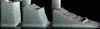 |
Fig. 1 Collapse of a granular column: image from the laboratory of a quasi-2D configuration from [17]. |
2 The granular collapse
Among the granular flow configurations for which the μ(I) rheology has been shown to be applicable, the granular collapse is particularly attractive due to its experimental accessibility and simplicity. It constitutes a well-controlled flow configuration that can be reproduced in laboratory experiments [17,18] or simulated numerically [19]. It consists of an initially confined column of grains that is suddenly released and allowed to spread under gravity over a horizontal surface (Fig. 1).
In this study, the flow is modeled in a two-dimensional (2D) configuration (Fig. 2), as it is assumed to be uniform along the z direction. The training data for the PINN model were generated using the two-phase flow solver Basilisk [20], which employs a Volume-of-Fluid (VOF) method to track the interface between air and the granular material. A series of numerical simulations were conducted in which the rheological parameters μs and μ2 were varied within prescribed ranges ( and
and  ). The flow variables are computed on a hierarchical octree mesh and subsequently interpolated onto a uniform 128 × 128 grid for database generation. Each point in the grid that lies within the granular material, i.e. where the VOF function c is strictly equal to 1, is associated with a spatial location (xi, yi) and a time coordinate ti, for which the velocity components (u, v) are known. The set of all such spatio-temporal points defines the velocity training dataset, denoted as
  .
.
For the pressure field, only the values at the interface between the granular material and the surrounding air are retained. Interface points are identified using the VOF function, namely where c = 0.5. Such values would typically be accessible in an experimental setting. Pressure values are assigned exclusively to these interface points during training. This subset of points constitutes the training dataset for pressure, denoted as Xsurf.
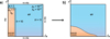 |
Fig. 2 Sketch of the 2D configuration of the granular column collapse at: a) the initial state; b) the final state. |
3 The PINN model
The PINN model (Fig. 3) is built upon a standard artificial neural network (ANN) that takes as input two spatial coordinates (x, y) and a temporal coordinate t, and outputs the corresponding components of the velocity field (u, v) and the pressure p.
To incorporate physical constraints, the derivatives of the predicted fields are computed via automatic differentiation [21], and used to evaluate the residuals of the governing equations, the Navier–Stokes equations, and the continuity equation:
 (3)
(3)
 (4)
(4)
where g = (0,−1) denotes the reduced gravity field and ηg the equivalent viscosity given by the μ(I)-rheology:
 (5)
(5)
Thus, unlike a conventional neural network, the loss function in a PINN does not rely solely on the discrepancies between the predicted and observed outputs (e0). Instead, it incorporates both a data mismatch term and a physics-based residual term. The total loss function is defined as follows:
 (6)
(6)
The equation residuals are included in the loss term 𝐿res, which penalizes deviations from the governing equations at a set of collocation points Xres. While these points can in principle be chosen arbitrarily, they are taken to coincide with the data points in this study, i.e.,  . The loss term is defined as:
 (7)
(7)
where eu, ev, and econt denote the residuals of the governing equations, i.e., the left-hand sides of equations (3) and (4).
The term 𝐿data in equation (6) accounts for the difference between the network predictions and the available training data, following the structure of a standard supervised loss function:
 (8)
(8)
where u𝒩(x), v𝒩(x) and psurf, 𝒩(x) denotes the predictions at point x in Xdata or Xsurf, the training datasets defined in Section 2, and ux, vx and psurf, x are the corresponding reference values at point x.
During training, the neural network parameters are updated to minimize the total loss function 𝐿tot. In order to identify the rheological parameters μs and μ2 of the μ(I) model, two additional trainable variables are introduced alongside the neural network’s weights and biases (Fig. 3). The overall optimization problem can therefore be formulated as follows:
 (9)
(9)
where Θ* denotes the optimized neural network’s parameters, and μs*, μ2* the identified values of the rheological parameters.
 |
Fig. 3 Representation of the PINN architecture used in this study. The neural network 𝒩 typically consists of three hidden layers with 250 neurons each. Automatic differentiation is used to compute derivatives of the predicted fields, which are then used to evaluate the residuals of the governing equations. Two additional trainable variables are initialized alongside the neural network’s parameters in order to identify the values of μs and μ2. |
4 Results
In this section, we present the results obtained using the PINN model applied to the granular column collapse configuration. We assess the model’s ability to accurately identify the rheological parameters μs and μ2 of the μ(I) rheology and to reconstruct the pressure field.
To this end, a set of neural networks was trained, with one network trained for each flow configuration. Training was performed for 2000 epochs on an Nvidia RTX A5000 GPU with a batch size of 512, while the learning rate was gradually decreased from 5 × 10⁻⁴ to 1 × 10⁻⁵. All networks shared the same architecture, consisting of three hidden layers of 250 neurons. The optimizer was Adam [22] and the swish activation function [23] was used in all layers except the output layer, which had no activation function.
To quantitatively evaluate the accuracy of the predicted fields and the identified parameters, we compute the relative L2 norm between the PINN predictions and the reference data. For the pressure field p, the relative L2 norm is defined as:
 (10)
(10)
where p𝒩(x) is the value predicted by the model at point x, and px is the corresponding reference value. This error is expressed as a percentage to facilitate interpretation. The same metric is also employed to assess the accuracy of the identified scalar parameters, μs and μ2.
4.1 Identification of μs and μ2
In order to obtain the best possible parameter identification results, we investigated the influence of the choice of observation points Xdata used to train the PINN. In particular, we tested different distributions of Xdata to assess whether concentrating observations in regions where the flow is active and strain-rate gradients are large could improve the identification of the rheological parameters. Figure 4 shows the evolution of the identified parameters μs (left) and μ2 (right) over the training epochs for several choices of observation point distributions. The points are either taken from the full uniform computational grid defined in Section 2 or sampled according to a probability law weighted by the maximum absolute value of D2.
Although all sampling strategies ultimately lead to comparable final values of μs and μ2, slight differences appear in the convergence behavior. In particular, μ2 typically requires more iterations to converge, which makes it important to ensure the proper convergence of both parameters. In this context, the case using the full uniform grid exhibits the fastest and most stable convergence. In addition, using the full grid leads to a significantly better reconstruction of the pressure field, which is particularly important in the multitask setting considered here, where both parameter identification and pressure reconstruction must be accurately achieved. Consequently, the results presented in the following are obtained from models trained using observation points distributed over the full uniform grid.
Table 1 summarizes the results obtained from the PINN-based parameter identification procedure for various combinations of the true values of μs and μ2. Overall, the model demonstrates robust performance in retrieving both parameters, with relative errors consistently below 2% for μs, and typically below 5% for μ2. The identification of μs appears particularly robust, with errors rarely exceeding 1.5%, even across a broad range of values from 0.2 to 0.6. The identification of μ2 shows slightly more variation, with errors ranging from approximately 1% to 7%, but remains well within acceptable bounds for practical applications. This confirms the ability of PINNs to accurately infer rheological properties from partial flow data, even when both parameters are learned simultaneously.
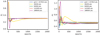 |
Fig. 4 Evolution of the identified rheological parameters μs (left) and μ2 (right) as a function of the training epochs for different numbers of observation points Xdata. Observation points are either taken from the full uniform computational grid (in blue) or sampled according to a probability distribution weighted by the maximum absolute value of D2. The dashed lines indicate the reference values of the identified parameters. |
Identification of rheological parameters and pressure reconstruction accuracy. Each row corresponds to a test case with given reference values of the rheological parameters μs and μ2. The table reports the values identified by the PINN model, the corresponding relative errors Òμs and Òμ2 (in percent), and the relative L2 norm error Òp (in percent) on the reconstructed pressure field.
4.2 Reconstruction of the pressure field
The last column of Table 1 reports the relative L2 norm for the reconstructed pressure field εp computed over the whole domain, for each test case. These errors are typically below 4%, indicating a high level of agreement between the PINN predictions and the reference pressure fields. The only exceptions occur for the largest values of μs and μ2, where the error increases to 7–8%, which may be attributed to the reduced sensitivity of the flow dynamics to the pressure distribution in these regimes or to numerical stiffness effects. Despite this slight increase, the accuracy remains acceptable, and the results confirm that the pressure field can be reliably reconstructed from velocity and limited interface pressure data using the PINN framework.
Figure 5 illustrates the comparison between the pressure field obtained from the CFD simulation using Basilisk (a) and the one reconstructed by the PINN model (b) at time t = 4.13 for μs = 0.3 and μ2 = 0.54. The two fields exhibit a good agreement, indicating that the PINN successfully captures the spatial structure of the pressure field. In panel (c), three pressure profiles along the x-direction are plotted for different fixed y-positions, highlighted by colored lines in panels (a) and (b). The profiles predicted by the PINN (dashed lines) closely follow those from the CFD data (solid lines). The overlap is particularly strong in the flowing regions of the granular material. Slight deviations are observed in the static zones, where the granular material does not flow. These discrepancies are expected, as the underlying rheological model and governing equations used by the PINN are not valid in these non-flowing regions.
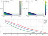 |
Fig. 5 At t = 4.13, for μs = 0.3 and μ2 = 0.54: a) the pressure field from Basilisk; b) the pressure field predicted by the PINN model; c) comparaison of three pressure profiles along the x-direction, the corresponding y coordinantes for the profiles are indicated in a) and b). |
5 Conclusion
We presented a first application of PINNs in the context of continuum modeling of granular materials, using the well-established μ(I)-rheology framework. By training the model on synthetic data of a simple granular column collapse, we showed that PINNs can accurately reconstruct the pressure field and identify key rheological parameters μs and μ2 with high precision. A key advantage of this approach lies in its ability to infer hard-to-measure physical quantities using only limited, easily accessible data, such as velocity fields and surface pressure. Our results suggest that PINNs provide a promising, flexible tool for rheological characterization of granular materials, especially in contexts where experimental measurements are limited or costly. Future work will focus on extending this approach to real experimental data, as well as to more complex granular configurations.
Funding
A part of this study is conducted in the framework of the Agence Nationale de la Recherche (Project ‘Pinn’terfaces’ ANR-23-CE23-0020).
Conflicts of interest
The authors have nothing to declare.
Data availabily statement
Data will be made available on request.
Author contributions statement
Barbara Baldoni: Conceptualization, Data Curation, Investigation, Methodology, Software, Validation, Visualization, Writing - Original Draft. Mickaël Delcey: Methodology, Software. Yoann Cheny: Conceptualization, Funding acquisition, Methodology, Supervision, Writing - Original Draft, Writing & Review & Editing. Adrien Gans: Data Curation, Methodology, Writing & Review & Editing. Mathieu Jenny: Writing & Review & Editing. Sébastien Kiesgen de Richter: Writing & Review & Editing.
References
- B. Andreotti, Y. Forterre, O. Pouliquen, Granular Media: Between Fluid and Solid, Cambridge University Press, 2013 [Google Scholar]
- M. Ouriemi, P. Aussillous, E. Guazzelli, Sediment dynamics. part 1. bed-load transport by laminar shearing flows, J. Fluid Mech. 636, 295–319 (2009) [Google Scholar]
- Y. Forterre, O. Pouliquen, Flows of dense granular media, Annu. Rev. Fluid Mech. 40, 1–24 (2008) [Google Scholar]
- D. Schulze, Powders and Bulk Solids: Behavior, Characterization, Storage and Flow, Springer, 2008 [Google Scholar]
- C. Allenspach, P. Timmins, G. Lumay, J. Holman, T. Minko, Loss-in-weight feeding, powder flow and electrostatic evaluation for direct compression hydroxypropyl methylcellulose (hpmc) to support continuous manufacturing, Int. J. Pharm. 596, 120259 (2021) [Google Scholar]
- J.v.d. Visser, Van der waals and other cohesive forces affecting powder fluidization, Powder Technol. 58, 1–10 (1989) [Google Scholar]
- S. Deboeuf, A. Fall, Cohesion and aggregates in unsaturated wet granular flows down a rough incline, J. Rheol. 67, 909–909 (2023) [Google Scholar]
- P.A. Cundall, O. Strack, A discrete numerical model for granular assemblies, Geotechnique 29, 47–65 (1979) [CrossRef] [Google Scholar]
- P. Jop, Y. Forterre, O. Pouliquen, A constitutive law for dense granular flows, Nature 441, 727–730 (2006) [NASA ADS] [CrossRef] [Google Scholar]
- M. Raissi, G.E. Karniadakis, Hidden physics models: machine learning of nonlinear partial differential equations, J. Comput. Phys. 357, 125–141 (2018) [NASA ADS] [CrossRef] [Google Scholar]
- G.E. Karniadakis, I.G. Kevrekidis, L. Lu, P. Perdikaris, S. Wang, L. Yang, Physics-informed machine learning, Nat. Rev. Phys. 3, 422–440 (2021) [Google Scholar]
- S.W. Kim, I. Kim, J. Lee, S. Lee, Knowledge integration into deep learning in dynamical systems: an overview and taxonomy, J. Mech. Sci. Technol. 35, 1331–1342 (2021) [Google Scholar]
- S. Cuomo, V.S. Di Cola, F. Giampaolo, G. Rozza, M. Raissi, F. Piccialli, Scientific machine learning through physics-informed neural[CE1] networks: where we are and what’s next, J. Sci. Comput. 92, (2022) [Google Scholar]
- S. Cai, Z. Wang, S. Wang, P. Perdikaris, G.E. Karniadakis, Physics-informed neural networks for heat transfer problems, J. Heat Transf. 143, (2021) [Google Scholar]
- M. Delcey, Y. Cheny, S.K. de Richter, Physics-informed neural networks for gravity currents reconstruction from limited data, Phys. Fluids (2022) [Google Scholar]
- C. Pan, S. Feng, S. Tao, H. Zhang, Y. Zheng, H. Ye, Physics-informed neural network for solving young–laplace equation and identifying parameters, Phys. Fluids 36, 022116 (2024) [Google Scholar]
- A. Gans, A. Abramian, P.-Y. Lagrée, M. Gong, A. Sauret, O. Pouliquen, M. Nicolas, Collapse of a cohesive granular column, J. Fluid Mech. 959, A41 (2023) [Google Scholar]
- E. Lajeunesse, J. Monnier, G. Homsy, Granular slumping on a horizontal surface, Phys. Fluids 17, (2005) [Google Scholar]
- L. Staron, E. Hinch, Study of the collapse of granular columns using two-dimensional discrete-grain simulation, J. Fluid Mech. 545, 1–27 (2005) [Google Scholar]
- S. Popinet, An accurate adaptive solver for surface-tension-driven interfacial flows, J. Comput. Phys. 228, 5838–5866 (2009) [CrossRef] [MathSciNet] [Google Scholar]
- A.G. Baydin, B.A. Pearlmutter, A.A. Radul, J.M. Siskind, Automatic differentiation in machine learning: a survey, J. Mach. Learn. Res. 18, 1–43 (2018) [Google Scholar]
- D.P. Kingma, J. Ba, Adam: a method for stochastic optimization, arXiv preprint arXiv:1412.6980 (2014) [Google Scholar]
- P. Ramachandran, B. Zoph, Q.V. Le, Searching for activation functions, arXiv preprint arXiv:1710.05941 (2017) [Google Scholar]
Cite this article as: B. Baldoni, M. Delcey, Y. Cheny, A. Gans, M. Jenny, S. Kiesgen de Richte, Physics-informed neural networks for granular flows modelling, Mechanics & Industry 27, 28 (2026), https://doi.org/10.1051/meca/2026027
All Tables
Identification of rheological parameters and pressure reconstruction accuracy. Each row corresponds to a test case with given reference values of the rheological parameters μs and μ2. The table reports the values identified by the PINN model, the corresponding relative errors Òμs and Òμ2 (in percent), and the relative L2 norm error Òp (in percent) on the reconstructed pressure field.
All Figures
|
Fig. 1 Collapse of a granular column: image from the laboratory of a quasi-2D configuration from [17]. |
| In the text | |
|
Fig. 2 Sketch of the 2D configuration of the granular column collapse at: a) the initial state; b) the final state. |
| In the text | |
|
Fig. 3 Representation of the PINN architecture used in this study. The neural network 𝒩 typically consists of three hidden layers with 250 neurons each. Automatic differentiation is used to compute derivatives of the predicted fields, which are then used to evaluate the residuals of the governing equations. Two additional trainable variables are initialized alongside the neural network’s parameters in order to identify the values of μs and μ2. |
| In the text | |
|
Fig. 4 Evolution of the identified rheological parameters μs (left) and μ2 (right) as a function of the training epochs for different numbers of observation points Xdata. Observation points are either taken from the full uniform computational grid (in blue) or sampled according to a probability distribution weighted by the maximum absolute value of D2. The dashed lines indicate the reference values of the identified parameters. |
| In the text | |
|
Fig. 5 At t = 4.13, for μs = 0.3 and μ2 = 0.54: a) the pressure field from Basilisk; b) the pressure field predicted by the PINN model; c) comparaison of three pressure profiles along the x-direction, the corresponding y coordinantes for the profiles are indicated in a) and b). |
| In the text | |
Current usage metrics show cumulative count of Article Views (full-text article views including HTML views, PDF and ePub downloads, according to the available data) and Abstracts Views on Vision4Press platform.
Data correspond to usage on the plateform after 2015. The current usage metrics is available 48-96 hours after online publication and is updated daily on week days.
Initial download of the metrics may take a while.