| Issue |
Mechanics & Industry
Volume 22, 2021
|
|
|---|---|---|
| Article Number | 22 | |
| Number of page(s) | 15 | |
| DOI | https://doi.org/10.1051/meca/2021023 | |
| Published online | 02 April 2021 | |
Regular Article
Optimal design to control rotor shaft vibrations and thermal management on a supercritical CO2 microturbine
1
School of Mechatronics Engineering, Henan University of Science and Technology, Henan Key Laboratory for Machinery Design and Transmission System, Henan University of Science and Technology, Luoyang, Henan 471003, PR China
2
School of Mechanical and Mining Engineering, University of Queensland, Brisbane, Australia
* e-mail: This email address is being protected from spambots. You need JavaScript enabled to view it.
Received:
18
September
2020
Accepted:
8
March
2021
Abstract
Supercritical carbon dioxide (SCO2) Brayton cycle microturbine can be used for the next generation of solar power. In order to comprehensively optimize the supporting system and cooling device parameters of Brayton cycle shafting, the concept of chaos interval is introduced by chaotic mapping, and the CIMPSO algorithm is proposed to optimize the multi-objective rotor system model with nonlinear variables.The results show that the resonance amplitude of the optimized model is effectively attenuated, and the critical speed point is far away from the working speed, which shows the robustness of the optimization algorithm. Finally, based on arbitrary several sets of optimization solutions and empirical parameters, the finite element model of shafting is established for simulation, and the results show that the optimized solution has certain guiding significance for the design of the rotor system.The cooling device is designed and simulated by CFD method based on the optimal solution set. Both the inlet boundary conditions of given pressure (1 MPα) and given mass flow rate (0.1 kg/s) numerical calculations were carried out to characterize the cooling performance, for different jet impingement configurations (Hr/din = 0.0125 ∼ 5).Several sets of analyses show the strong effects of the jet-to-target spacing (Hr/din) on the rotor thermal performance at a given diameter (din) of the nozzle. Average temperature (Tc) at the free end of the rotor show that, as jet-to-target distance decreases (0.0125 ≤ Hr/din ≤ 0.33), the heat dissipation efficiency of the cooling device with the given pressure boundary condition tends to decrease, while the conclusion is opposite when the inlet boundary condition is set to the given mass flow rate. And there is an interval for the optimal combination (Hr/din) to promote the cooling efficiency.
Key words: Multi-objective optimization / particle swarm / thermal management / rotor dynamics
© J. Li et al., Published by EDP Sciences 2021
 This is an Open Access article distributed under the terms of the Creative Commons Attribution License (https://creativecommons.org/licenses/by/4.0), which permits unrestricted use, distribution, and reproduction in any medium, provided the original work is properly cited.
1 Introduction
Supercritical CO2 Brayton cycle is proposed as the next-generation technology in a diverse range of applications including nuclear power generation, fossil fuel power generation, and concentrated solar power [1,2]. Thermodynamic energy conversion system is the key issue in the future power generation. As described in the relevant literature [3], under the condition that the inlet temperature of the turbine is greater than 550 ° C, the ultra-supercritical (USC) steam cycle steam is demanded to improve the efficiency of the traditional Rankine cycle which has been widely utilized over the past decades, but the USC may interact with structural materials to create a potential threat to the circulation system.As the turbine inlet temperature gets higher, the steam cycle in any form becomes even less suitable. Compared with steam at the same temperature, the SCO2 has the advantages of less corrosion and less work required for compression. As a result, the SCO2 Brayton cycle can be considered as an alternative power conversion system, which can operate at high inlet turbine temperatures in a safe and reliable fashion [3,4].
The CO2 fluid becomes approximately incompressible near the critical point (30.98 ° C and 7.38 MPa), allowing it has a very high power density in supercritical state leading to compact footprint, small turbomachinery and micro-channel heat exchangers are capitalized in SCO2 cycles [5]. There has been significant research focus on SCO2 Brayton cycle for the next generation nuclear reactor systems and other power plants. Most of the investigations have been theoretical including thermodynamic cycle optimization directed towards determination of the optimum cycle lay-outs in different applications. Some higher fidelity numerical simulations using computational fluid dynamic (CFD) have been conducted modelling components of Brayton cycles, such as heat conduction medium, turbine, and heat receiver [6–10].
Recent interest in supercritical CO2 cycles has been mostly directed at large-scale power generation using utility-scale axial turbines, e.g. in coal fired power generation with carbon capture and nuclear power generation. SCO2 cycles can also enable modular scalable and efficient Concentrating Solar Thermal (CST) power generation with storage [11–13]. Average cost of electricity from combined CST + PV solar power generators would be cheaper than diesel generation and would offer day and night affordable electricity to communities around the world unconnected to national power grids. The focus of this paper is on SCO2 radial-in-flow turbines suitable for small-scale power generation at turbine sizes from 0.3 to 30 MWe. As mentioned above, the immediate market for this type of turbine is off-grid power generation using CST with thermal storage.
As shown in Figure 1 our proposed radial-in-flow turbine configuration for a SCO2 cycle employs an overhung shaft supported by two bearings, which use conventional technology (hydrodynamic or magnetic bearings). The reason for using an overhung shaft is to protect the two off-the-shelf bearings against the high-temperature high-pressure cycle fluid using at least two seals. This overhung configuration coupled with very high rotational speeds pose a significant challenge in terms of shaft vibrations. The University of Queensland and Henan University of Science and Technology have a joint project investigating design options to control vibrations and rotor Thermal conduction management for this configuration. The following options are being considered for the two radial bearings:
-
Magnetic bearings with controllable support stiffness and damping
-
Oil-lubricated tilted pad bearings in rigid hubs
-
Oil-lubricated tilted pad bearings in compliant hubs
At these high rotational speeds, the expected life in operating hours will be limited for rolling-element bearings. Therefore, they are not considered in this study. The analysis will be conducted for a 300-kWe rotor supported by Oil-lubricated tilted pad bearings in compliant hubs rotating at a speed of 50000 RPM. The low end of the power range is used because small SCO2 turbines offer the greatest challenge in terms of shaft dynamics due to their high rotational speed. The optimum shaft speed gets lower as the turbines get larger [8].
For the purpose of this study, the rotor geometry is represented as shown in Figure 2. The lengths of the labyrinth seal, the cooling zone, the DGS are constrained by other requirements. For example, the length of the labyrinth seal is constrained by leakage considerations; the cooling zone needs to be long enough to cool the rotor shaft to a temperature the DGS can tolerate; the length of the DGS section is determined by the seal manufacturer's design. The values given in the table are reasonable approximations of the actual values. The bearing spacing is also expressed as bD and the effect of varying b on shaft dynamics will be examined as the main constraint on bearing spacing is placed by shaft dynamics, which is the topic of the present study. The cooling device is used to prevent blade temperatures from affecting the rotor support system and to improve cantilever stiffness as a gas bearing. The necessary first step in cooling device design is the prediction of the dynamic characteristics: based on the harmonic response of rotor dynamics, the vibration mass, stiffness and damping of the compliant hubs, and stiffness coefficient of the cooling device are optimized by multi-objective numerical calculation. The design of the cooling device was executed by employing a three-dimensional CFD-based methodology while the performance and efficiency of the cooling device were investigated.
 |
Fig. 1 Supercritical CO2 radial-in-flow turbine lay-out. |
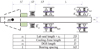 |
Fig. 2 Approximate rotor shaft geometry. |
2 Optimal design of rotor system
2.1 Rotor system structure
In the turbine rotor system shown in Figure 2, the composite stiffness and damping of the main support with a distance of L can be expressed as [14]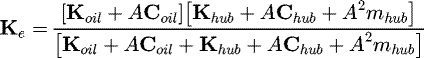 (1)
(1)
For tilting pad bearing support system with flexible bearing pedestal,
K
oil
and C
oil are the stiffness and damping matrix of the bearing respectively. K
hub and C
hub are the stiffness and damping matrix of the bearing pedestal respectively. The whirl frequency of rotor is expressed as complex number (2)
(2)
The diameter of the rotor is D, and the bearing spacing is defined as (3)
(3)
where parameter b is the coefficient to be optimized. S1, S2 and S3 are axial dimensions of impeller, cooling device and sealing mechanism respectively. The lubricating medium for cooling deviceis SCO2. As an auxiliary support, its stiffness is a nonlinear function of rotor speed (n) and rotor displacement (s), which can be expressed as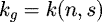 (4)
(4)
In order to establish the finite element and transfer matrix model, the impeller is equivalent to a rigid disc with diameter d = 100 mm and thickness h = 10 mm, and the mass of the disc is 0.71 kg. The reason for this equivalent operation is that the disc and impeller have the same diameter and pole moment of inertia.
2.2 Objective function of rotor system optimization
The cooling and supporting parameters of the shafting of the SCO2 solar generator directly affect its critical speed and the amplitude of the imbalanced response. Therefore, the bearing spacing L, the stiffness khub, the damping chub and the mass mhub of the bearing pedestal, and the stiffness  of the cooling device are taken as the input variables of the system to be optimized. The mathematical model of rotor system can be established by the classical Riccati transfer matrix method [14]. The rotor is divided into several disc-axis elements, and the relation between any two adjacent cross sections can be described as
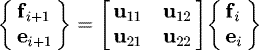 (5)
(5)
where the output parameters e and f are the internal forces (bending moment and shear force) of the plural trajectory and section respectively. The u is the transfer matrix corresponding to the disc-axis element. A detailed introduction of the transfer matrix can be found in reference [14]. Rotor system design is a multi-objective optimization problem, which can be used as fitness evaluation functions including.
-
The maximum peak of the unbalance response of the rotor
 (6)
(6)
The  in the formula can be obtained from the complex parameter e
i of the current node.
in the formula can be obtained from the complex parameter e
i of the current node.
-
The absolute value of the difference between the operating speed and the nearest critical speed
 (7)
(7)
Where, ncritical is the critical frequency closest to the operating frequency nwork.
-
The derivative of the amplitude of the unbalance response at the working speed point to the frequency
 (8)
(8)
In the actual numerical calculation, it can be written as a difference form:
where, An+1 and An−1 respectively represent the amplitude of the unbalanced response at the rotational speed point adjacent to the operating frequency point, which can also be obtained from the complex vibration parameter e i.
The fitness function of constraint optimization can be written as (9)
(9)
A certain space is reserved for the output part while ensuring the stiffness of the rotor. Therefore, the constraint range of parameter b is (10)
(10)
The constraint range of relevant parameters of bearing pedestal can be taken as (11)
(11)
where,  and
and  are respectively the Maximum stiffness and Maximum damping of the tilting tile bearing at working speed, and s is the scaling factor. The stiffness of SCO2 cooling device is a nonlinear function of rotor speed and displacement. In practical application, the stiffness of gas bearing can be constrained as
 (12)
(12)
where, Kupper is the upper limit of gas bearing stiffness in practical application, which is determined by the pressure of lubricating medium and design parameters ofbearings. In rotor dynamics, for every harmonic response analysis, the stiffness of gas bearing brought into the system is a two-dimensional matrix related to speed and rotor displacement. Due to the nonlinearity of gas film stiffness, the stiffness of cooling device is unknown during numerical analysis. This brings challenges to the application of conventional genetic algorithm, simulated annealing algorithm and particle swarm optimization algorithm in the optimization of shafting parameters. In order to deal with the above problems, a chaos interval multi-objective particle swarm optimization algorithm (CIMPSO) was proposed, and the rotor system parameters of the turbine are optimized.
Within the constraint range of stiffness of the cooling device, the characteristic number kge is taken as an element in the particle vector, and the chaos interval particle to be optimized can be described as (13)
(13)
2.3 Optimization of rotor system based on CIMPSO
Particle swarm optimization (PSO) is a kind of computing technology based on self-cognition and social psychology. Every potential feasible solution in optimization space is abstracted as a particle vector X
i. PSO starts with a random initial population in the constrained space, and each particle is defined by velocity and displacement. In the space, individual particles achieve information sharing mechanism while local optimization. The correct behavior of the particles is strengthened, while being imitated by other particles, and finally converges to the optimal solution or the non-inferior optimal target domain (Pareto front). The standard particle swarm optimization algorithm uses the following formula to iteratively update particles [15]: (14)
(14)
 (15)
(15)
Suppose the number of initialized particles is N, i = 1, 2..., N, means the sequence number of particles. The fitness of each particle is determined by the objective function f (t). In the iterative process, each particle remembers and tracks the current individual optimal particle P i (t) and the global optimal particle P g (t). wv and wx are inertial weight and forgetting inertial weight, which determine the global optimization ability of the algorithm.r1 and r2 are random numbers between 0 and 1, indicating the cognitive ability of the particle.c1 and c2 is the learning factor, indicating the learning ability of particles.
For the shafting in this paper, the stiffness of the cooling device is a two-dimensional nonlinear elements (DNE) that varies according to the rotation speed and displacement of the shaft. The values of stiffness elements are constrained by applications. Set the upper and lower limits of the constraints as (16)
(16)
where, α and β are expansion coefficients based on the characteristic number of particle elements. In order to achieve particle swarm optimization with DNE, chaos variables are introduced here. The logistic equation of a typical chaotic system [15] (17)can be used to obtain random chaotic variables. Chaotic variables have the characteristics of regularity, ergodicity and randomness in a certain range. Where, μ is the control parameter, zn ∈ (0, 1). After updating the particle X
i at each iteration step, the stiffness characteristic number kge of the cooling device is mapped to the Logistic equation to initialize the chaotic variables
(17)can be used to obtain random chaotic variables. Chaotic variables have the characteristics of regularity, ergodicity and randomness in a certain range. Where, μ is the control parameter, zn ∈ (0, 1). After updating the particle X
i at each iteration step, the stiffness characteristic number kge of the cooling device is mapped to the Logistic equation to initialize the chaotic variables (18)where, t represents the current iteration step. Substitute z1 (t) into Logistic equation for iteration to produce chaotic variable sequence zi+1 (t) (i = 1, 2, ⋯ N). The chaotic sequence zi+1 (t) is inversely mapped to the solution space to obtain
 (19)
(19)
 is used to replace the stiffness characteristic number in the current particle swarm, and a new input particle with chaotic characteristic is obtained
 (20)
(20)
where, i = 1, 2, ... , N represents the number of particles. The above mentioned iterative process of generating chaotic sequences from variables is called chaotic mapping, denoted as (21)
(21)
Particle swarm  with chaotic characteristics represents all possible stiffness coefficients determined by stiffness eigenvalues. This approach transforms the spatial complexity of the system into time complexity and then solves the non-inferior optimal target domain. The fitness of chaotic characteristic particle
  is calculated in solution space. Each particle was evaluated simultaneously with three fitness values A (t), Δn (t) and ADC (t), corresponding to three individual historical optimal particles
  ,
,  and
and  respectively. Then, perform fast non-dominated sorting is performed on the fitness value, and the global optimal particle is selected from the first-order particles, denoted as
 (22)
(22)
where, M fit (⋅) refers to the particle with the Comprehensive optimal fitness in the current iteration. Sub-objective function normalization: (23)
(23)
 (24)
(24)
 (25)
(25)
The comprehensive fitness value of each individual particle was obtained by (26)Where, ϕk represent the optimal particle weight factor, and ϕ1 + ϕ2 + ϕ3 = 1, i is the number of particle.
In the multi-objective optimization problem of rotor system, each fitness function may be gamed against each other, so every time the particle fitness is evaluated, the optimal solution for degradation needs to be eliminated. The particle  ,
,  and
and  with the worst fitness values of A (t), Δn (t) and ADC (t) in the current iteration step are respectively searched. Three new random particles are obtained by chaos mapping the global optimal particle P
g (t), and the worst particle is replaced
with the worst fitness values of A (t), Δn (t) and ADC (t) in the current iteration step are respectively searched. Three new random particles are obtained by chaos mapping the global optimal particle P
g (t), and the worst particle is replaced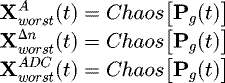 (27)
(27)
In the current iteration step, kge (t) is still used as the element of the stiffness characteristic number of the replaced particles. Finally, new particles are iteratively obtained according to standard particle swarm optimization (Eqs. (14) and (15)) algorithm: (28)
(28)
The optimization method described above is called chaotic intervalmulti-objective particle swarm optimization algorithm (CIMPSO). Compared with the standard chaotic particle swarm optimization (ChPSO) algorithm, the CIMPSO proposed in this paper can perform spatial optimization for multi-objective particle swarm models with two-dimensional nonlinear elements. When individual and global optimal particles do not evolve with iterations, then each particle of the particle swarm updates independently, and finally all particles tend to the global optimal solution or non-inferior optimal solution. However, all particles in the particle swarm contain chaotic maps with Characteristic number elements, which ensures effective optimization calculation of the interval of chaos interval elements within the range of chaotic maps. The convergence test for CIMPSO is in Appendix 1.
2.4 Induction of CIMPSO algorithm
The linearized oil film force model of oil-lubricated bearings is suitable for rotor micro-vibration. Some rotating machinery has the characteristics of high speed, lowflexibility and large span, however. The linear stiffness model based on small disturbance may have a large deviation from the actual situation. The rotor may exhibit nonlinear dynamic behavior under the action of nonlinear oil film force. In the process of dealing with the optimization problem of high-speed rotor systems, the main difficulty faced is the nonlinearity of the parameters such as the stiffness of the oil-lubricated bearings and the cooling device. The main advantage of CIMPSO isthat chaotic mapping is introduced to solve the problem of multi-objective optimization with nonlinear elements, the pseudo code of the algorithm is shown in Table 1. Based on the optimization process of the rotor system, the algorithm is mainly divided into the following steps.
Step 1: Initialize relevant parameters, including learning factor c1 and c2, particle swarm size N, optimization times T, velocity inertia weight wv and position inertia weight wx, expansion coefficient α and β, control parameters μ.
Step 2: All particle positions are randomly initialized within the constraint range. The position of the particle is denoted as X
i (t, j)(j represents the position number of the nonlinear element in the particle vector X, t represents the number of iteration steps). Determine the characteristic number X
i (t, c) of the nonlinear element in the particle vector. The X
i (t, c) is substituted into the Equation (21) to generate the chaotic variable sequenceand replace the characteristic number elements in all particle vectors:
Step 3: Calculate the fitness of the particle vector. Each fitness corresponds to a historical individual optimal value of the particle, denoted as  ,
, ,…
,… (Assume that the number of objective functions is k). Perform non-dominated sorting on all individual optimal values of the current iteration step to obtain the first dominance layer particle swarm.
According to the operator's preference, the particle with the best fitness is selected from the first dominating layer as the global optimal particle.
Step 4: Generate a sequence of chaotic variables: where, k is the number of the objective function. Respectively replace the particles with the worst fitness that the decision maker considers in the current iteration step with the chaotic variable
  . The characteristic number element of each particle remains unchanged. Finally, the particle vector is updated iteratively according to the standard particle swarm optimization algorithm equations (14) and (15).
Pseudo code of the CIMPSO algorithm.
2.5 Optimal calculation
As mentioned above, the parameters to be optimized for the rotor system of the SCO2 turbine include the bearing spacing L = Db of the main supporting system, the mass mhub, stiffness khub and damping chub of bearing pedestal, and the stiffness  of cooling device. Where
  is a chaos interval element, namely anonlinear function of rotor speed and displacement, and its characteristic number is kge. The constraint condition of each element is
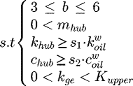 (29)where,
 and
and  are the stiffness and damping coefficient of the tilting pad bearing at working speed respectively. And, s1 = s2 = 0.8,Kupper = 1 × 10⁷ N/m. A chaotic interval multi-objective particle swarm model was established, and parameter initialization was shown in Table 2. The particles were randomly initialized in the constraint space, and five groups of results were randomly selected after repeated optimization calculations, as shown in Table 3. The average particle
  is obtained from the element average of all the optimized particles.
With reference to design experience, the bearing spacing is 3–5 times the diameter of the rotator, and the distance here is 3. The vibration mass of the bearing pedestal is half of the rotor mass (2.49 kg), In this analysis, the mass is 1.2 kg; The stiffness of the bearing hubs is half of the tilting pad bearing's, and the damping coefficient is equal to that of the tilting pad bearing; The stiffness of the gas bearing takes the middle value of the constraint space. Then the empirical particle parameter is (30)
(30)
The particles were randomly initialized in the constraint space, and optimized for 25 times consecutively. Each time, the objective function was evaluated 200 times, and 25 groups of non-inferior optimal solutions were obtained. The unbalanced response generated by bringing the 25 groups of non-inferior optimal solutions into the rotor system are shown as the solid lines in the Figure 3. The dot-dash line shown in the figure represents the unbalanced response of the rotor system with empirical particle X e, and the imbalanced response of the rotor calculated with the non-inferior optimal particles are shown as the solid lines. It can be seen from the figure that the relative peak value before optimization is 13.73 − 1.94 = 11.79. The imbalanced response of the rotor calculated with the non-inferior optimal particles in Table 3 is shown as the solid line in Figure 3. Compared with the dashed-dotted line, the solid line shows a minimum peak attenuation rate of 68.3%, and the response curve is more gentle, which reflects the robustness of CIMPSO algorithm. The difference between the working speed (nwork) and the nearest critical speed accounts for about 30% of the nwork, which ensures that the rotor works in a smooth steady whirling region.
Particle swarm model parameters.
Optimized parameters.
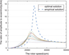 |
Fig. 3 Rotor imbalance response before and after optimization design. |
3 Design of cooling device
3.1 Geometrical configuration of cooling device
If a larger stiffness coefficient of bearing pedestal is required, particle X 1 in Table 3 can be used as the final optimization parameter. According to equation (16), the acceptable range of stiffness kcb of the cooling device is optimized space [1.37 × 10⁵, 2.53 × 10⁵]. The orifice restrictor has been often employed in actual gas bearings, because of its simplicity. The cooling device detailed in Figure 4 is designed for operation at high rotor speed (maximum of 60 krpm) and with impeller temperatures to a maximum of 873 K. The entire cooling device is divided into two hydrostatic zones by the pressure relief groove, which act on the two nodes of the shaft respectively. Each zone has eight equally distributed orifices. In addition, the pressure relief groove with eight inlets connected to the discharge channel to avoid the cross stiffness caused by the dynamic pressure effect and to increase heat dissipation capacity.
In order to prevent the shaft being stuck due to thermal expansion in the shutdown stateand over positioning, the radius clearancebetween the cooling device and the shaft is set to a larger value cr = 0.05 mm. For lubrication flow, Reynolds number is [16] (31)where u = 78.54 m/s is the rotor working speed and L2 = 10 mm is the width of the hydrostatic zones. Consider the extreme case: the density and dynamic viscosity of CO2 near the critical state are ρc = 467.6 kg/m3 and μc = 2.88 × 10⁻⁵ pa ⋅ s, respectively. The value of equation (29) is derived as Re = 318.8, which is less than the critical Reynolds number [16] Rc = 1000 of the eccentric ring. Even under extreme operating conditions.
The distance from the geometric center of the rotor to the geometric center of the cooling device is recorded as ec. In a later section of this paper, the cooling device was designed, and its dynamic characteristics and thermal management were simulated. The carbon dioxide in the radial clearance of hydrostatic zones is still in laminar flow. Table 4 shows the other principal dimensions of SCO2 cooling devices treated in this paper.
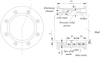 |
Fig. 4 SCO2 cooling devices treated in this paper. |
Principal dimensions treated in this paper.
3.2 Orifice diameter of cooling devices
To numerically obtain the static and dynamic characteristics, CFD are employed to predict experimental stiffness coefficients. In this paper, the commercial software Fluent were adopted to calculate the stiffness coefficients. The pressure relief groove in Figure 4 communicates with the atmosphere, therefore the pressure at the hydrostatic zone ends in the radial direction is set to the ambient pressure. The initial pressure boundary conditions at the entrance of the inlet hole is given, and assuming the pressure ps is 7 MPa.
Figure 5 depicts the recorded dynamic stiffness coefficients versus orifices with diameters of 0.1, 0.15 and 0.2 mm. Different from the conventional fluid lubricated bearing [14], the dynamic pressure effect is minimized by the existence of the pressure relief groove. No significant effect on the stiffness of the cooling device are ascertained between the rotor speeds operating in the range of 0 to 60 krpm. In contrast, the stiffness coefficient of the cooling device changes with the increase of rotor displacement, due to the flow of the orifices is restricted by rotor surface. In the rotor system studied in this paper, the cooling device assumes auxiliary support and heat dissipation, but does not bear the load of the rotor. Note that the bearing capacity does not need to be considered. Therefore, according to optimization space kcb mentioned above and Figure 6, the diameter of the orifice should be between 0.1 and 0.15 mm. In the following study, the diameters ds are selected as 0.12 and 0.13 mm.
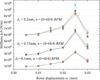 |
Fig. 5 Dynamic stiffness coefficient versus rotor displacement with different diameters ds. |
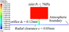 |
Fig. 6 Pressure distributions around an orifice obtained by CFD. |
3.3 Dynamic stiffness of cooling device
Figure 6 shows the pressure distributions of the hydrostatic zone. The supply pressure is 7 MPa, and the outlets are set to local atmospheric boundary. Thefigure depicts that the flow of carbon dioxide was mainly restricted at two places where pressure changes rapidly. One is at the entrance of the throttle orifice and the other is at the junction between the throttle orifice and the gap. The gas film at the junction and the throttling effect of the orifice together form the stiffness of the cooling device. Figure 7 shows the variation trend of the static and dynamic stiffness for the cooling device with orifice of 0.12 and 0.13 mm diameter. As indicated in this picture, the stiffness coefficient for rotor speed (n) values of 0 and 50 krpm that are given at the same ec were almost no change. With the increase of ec, the stiffness coefficient presents a nonlinear and complex tendency of variation.
Figure 8 shows the relationship between the stiffness coefficient (kcb) and mass flow (Q) of outlet with orifices of ds = 0.12 mm. The Q here refers to the mass flow rate of the orifice facing the direction of rotor displacement. When ec is less than 1.0 × 10⁻⁵ mm, the mass flow rate of the orifice remains unchanged, and the stiffness coefficient is also approximately a constant value. Under this condition, the stiffness of the bearing is the inherent rigidity of the CO2 gas film at the junction of the radius clearance and the throttle orifice, which is approximately linear. For 1.0 × 10⁵ m < ec < 2.5 × 10⁵ m, the stiffness coefficient gradually increases with thegradual decrease of mass flow. For ec > 2.5 × 10⁵ m, the bearing stiffness curve becomes tortuous because carbon dioxide flow was choked at the outlet of the orifice. As demonstrated in the figure, the mass flow rate of the orifice decreases rapidlyfor this stage.
In order to analyze and verify the influence of the stiffness of the gas bearing on the dynamic characteristics of the optimized rotor system, the inflection points K c (K c = [1.46E5, 1.88E5, 3.26E5, 3.46E5, 1.84E5, 8.02E5]) of the stiffness curve in Figure 8 were extracted. Replace the kge in X 1 with K c to obtain a new particle swarm X ci (i = length (K c)). The commercial software ANSYS was employed to establish the finite element model with particle swarm X ci and experience particle X e as the parameters. As shown in Figure 9 in the finite element three-dimensional model, the impeller is equivalent to a mass point with the same mass and moment of inertia. The effective vibration mass of the flexible bearing pedestal is mhub, which is shown as a circular hub in the figure. The inner and outer sides of the hub are virtual oil-lubricated tilted pad bearings and stiffness damping system respectively. The harmonic response analysis results of the finite element model for parameters X ci and X e are displayed in Figure 10, corresponding to the solid and dashed lines in the figure, respectively. Compared with the dashed line, the resonance peak corresponding to X ci has a significant attenuation, and the average attenuation rate is 60.7%. Furthermore, the results of the finite element analysis revealed that the value of K c was selected in a wider range based on the characteristic number kge, rather than limited to the optimization space (Eq. (16)), the resonance peak of the rotor system is still effectively controlled. Which further verifies the effectiveness and robustness of the optimized solution obtained by the CIMPSO algorithm.
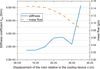 |
Fig. 7 Rotor displacement ec versus stiffness kcb. |
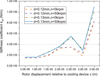 |
Fig. 8 Stiffness coefficient kcb versus mass flow rate Q of the orifice. |
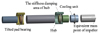 |
Fig. 9 Three-dimensional finite element model of the rotor system. |
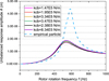 |
Fig. 10 Verify the effect of the stiffness coefficient of the gas bearing with orifice for ds = 0.12 mm on the synchronous responses of the rotor. |
3.4 Thermal management
Vertical impingements of single or an array of gas jet on the surface can increase the coefficient of convective heat transfer. To this end, for a fixed diameter of 30 mm rotating shaft, a set of different jet-to-target spacings (Hr/din = 0.0125 ∼ 5.0) were investigated, and for a fixed diameter of jet inlet (din) of 3 mm, three different impeller temperature of 873, 973, and 1073 K were investigated. Figure 2 depicts the current configuration of the cooling device and its structural diagram. There are eight inlet channels with diameter din evenly distributed in the circumferential direction of the cooling zone for supplying SCO2. Hr in the figure represents the radius gap of the pressure relief groove. High-density carbon dioxide (CO2) is injected into the pressure relief groove, and then recovered through the discharge channel. Note that the impeller acts as a steady source of thermal energy to heat the rotor-bearing system, and assuming that the temperature of the impeller is heated to 873 K and the supply pressure of CO2 at the inlet channel is 7 MPa. While considering the endothermic effect of gas in the expansion process, Figure 11 depicts the recorded temperature of CO2 versus free end temperature Tc of the rotor. The results reveal a evident reduction in the temperature of the free end relative to that of CO2 at the inlet with din = 3 mm and din = 4 mm, San Andres et al. obtained similar conclusions with experiments [17]. On the other hand, Figure 11a shows that an inlet channel with a diameter of din = 2 mm cannot supply sufficient flow to ensure that the free end temperature Tc equal to or lower than TCO2.
In SCO2 turbines, an effective thermal management strategy must be ascertained to maintain an acceptable temperature, not affecting significantly the material and lubricating medium properties of the bearings and avoiding axial excessive thermal gradients of the rotor. Therefore, CO2 of higher temperature should be selected as the cooling medium. The cooling device is divided into three zones: the cooling zone in the middle and the hydrostatic zones on both sides. The convective heat transfer occurs mainly in the wall jet area located in the cooling zone. As shown in Figure 12, the overall temperature distribution diagram with TCO2 = 350 K, the lowest temperature in the cooling zone islocated at the outlet (wall jet area). This indicates that the expansion and endothermic effect of high-density carbon dioxide needs to be carefully considered. Comparing with Figures 12a and b, the temperature gradient, over the whole shaft segment, increases because of the hydrostatic zone. The Figure 12c shows curves denoting the shaft segment temperature gradient with different orifice diameters. The solid line representing the rotor axis temperature in Figure 12b is regarded as a base line since the cooling device does not include any hydrostatic zone. The axial thermal gradient from the heated end toward the free end of the rotor increases due to the hydrostatic zone. The temperatures on free end, on the other hand, does not change significantly with the diameter ds of the orifice in the hydrostatic zone (Fig. 12).
In terms of geometry, the convective heat transfer coefficient is mainly affected by the jet-to-target spacing (hr = Hr/din), when the gas jet flows into the static environment from a circular section nozzle with a diameter of din. In order to investigate the influence of the dimensionless jet radius (Hr/din) of the cooling device on the cooling efficiency under the two boundary conditions of a given pressure and a given mass flow rate respectively, the cooling efficiency is evaluated by the temperature of the rotor after cooling. The endothermic effect of gas expansion and the influence of Hr/din can be considered in CFD calculation of thermal coupling analysis. It can be concluded from Figure 11 that the inlet with din ≥ 3mm can supply enough CO2 to take away the heat transferred from the impeller to the shaft. Therefore, the influence of gas flow on heat dissipation efficiency can be eliminated by setting din equal to or greater than 3mm. The heat dissipation efficiency was able to be quantified by the free endtemperature Tc.
Figure 13 concludes with the relative heat transfer performance of different configurations (Hr/din = 0.0125 ∼ 5.0) by comparing the average temperature (Tc) of the free end of the rotor. The above temperature parameter was chosen to signify the cooling effect of the cooling configuration for a given heat input (Ts) and nozzle boundary conditions. The inlet temperature of carbon dioxide at the nozzle is 320 K. At the different fixed Ts, Figure 13a depicts the temperature of the rotor after being impacted by the CO2 flow versus radius gap Hr. It is noted that the strong effects of the jet-to-target spacing on the rotor thermal performance at a given mass flow rate of the nozzle. In the interval 0.0125 < Hr/din < 0.07 configuration, the same coolant takes away more heat and makes the temperature of the rotor lower than otherwise. As a result, the temperature at free end for that the jet-to-target spacing was varied from 0.1 to 0 case decreases at a faster rate as compared to the larger jet gap (Hr), hence higher efficiency in heat transfer is expected for the much small jet gap configuration. However, the gain in heat transfer comes at a cost of increased pumping power in order to maintain the constant mass flow condition as the other configurations. With the variation of the Hr/din from 0.0125 to 5.0, after a fluctuation, Tc continues to increase approximately linearly until reaching the inflection point, and the inflection point is near Hr/din = 1. It can be inferred that the heat dissipation efficiency of the cooling device will no longer be significantly attenuated when Hr/din > 1, because after the inflection point, the value of Tc will no longer fluctuate significantly with the variation of Hr/din.
Globally averaged Temperature at the free end of the rotor has been plotted with respect to associated source temperatures (Ts = 873 K, Ts = 973 K, Ts = 1073K) for all the configurations in the range of 0.0125 ≤ Hr/din ≤ 5.0, as shown in Figure 13b. The cooling capacity have been studied for the given pressure of nozzle. Configurations with narrow jet spacings had higher flow resistance due to the presence of viscous force. In the range of 0.0125 < Hr/din ≤ 0.17, with increasing Hr/din, this CO2 flow resistance reduced, and the temperature at the free end of the rotor approached a linear decreasing trend. For the 0.17 < Hr/din ≤ 5, the temperature at the free end fluctuates only slightly, and overall it is close to the horizontal trend, therefore, the best combination of Hr/din should be within this range. This paragraph presents a comparative analysis between studies related to jet impingement onto rotor with a given mass flow rate and the studies that deals with jet impingement onto rotor under a given pressure. To this end, the mass flow rate of various jet-to-target spacing Hr/din configurations in the study were compared with the temperature Tc of the free end as shown in Figure 13b. Above configurations involving increased mass flow in significant enhancement in heat transfer when compared to the small jet-to-target spacing configuration.
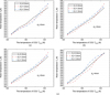 |
Fig. 11 The temperature of SCO2 versus free end temperature, calculation condition: (a) din = 2 mm, (b) din = 3 mm, (c) din = 4 mm. |
 |
Fig. 12 Temperature distribution cloud map and gradient comparison chart, din = 4 mm, Hg = 1.5 mm, TCO2 = 350 K, PCO2 = 7 MPa.(a) With hydrostatic zone. (b) No hydrostatic zone. (c) Temperature gradient comparison. |
 |
Fig. 13 Rotor temperature demonstrates that characteristic parameter Hr/din versus cooling efficiency, (a) Given mass flow (q = 0.1 kg/s) of nozzle, (b) Given pressure (1 MPa) of nozzle. |
4 Conclusions
Increasingly often in today's world of turbine design and development programs, stakeholders in rotor design desire the use of intelligent optimization algorithms in the design process. A primary reason is that intelligent optimization algorithm have been shown to optimize dynamic performance of rotor, such as reduced vibration and adjustment of critical frequency, more accurately and efficiently than Design experience. In this paper, a multi-objective optimization design is carried out for the rotor system of the SCO2 microturbine. Within this contribution an optimization design procedure of rotor system with emphasis ontwo nonlinear elements is proposed, and the chaotic interval particle swarm optimization (CIMPSO) algorithm is summarized.
This algorithm is used to optimize the rotor system of SCO2 turbine for multiple times, and the global non-inferior optimal or suboptimal solution sets are obtained. Commercial software ANSYS was used to establish a finite element model base on the solution sets for simulation verification. The results show that the resonance peaks of the rotor are effectively attenuated, and the critical speed is far away from the operating speed point, which verifies the robustness of the algorithm.
Demonstrated cooling device at high temperature is fundamental to enable the implementation of active magnetic bearing (AMB) and Oil-lubricated tilted pad bearings (OTB) into SCO2 turbines applications. The cooling device is simulated and the results revealed thatSCO2 cooling flow rates of high pressure character ensure an adequate thermal management for turbines operation at high temperatures. Determination of the high cooling efficiency for adequate thermal management is an issue of current research. For the coolant temperatures, six different jet-to-target spacing (Hr/din = 1/8, 1/6, 1/4, 1/3, 1/2, 3/4) were investigated, and for the fixed coolant temperature (TCO2 = 320K), two different nozzle boundary conditions of given inlet mass flow rate (q = 0.1 kg/s) and given inlet pressure (ps = 1 MPα) were investigated. Flow and thermal field computations are performed for the above two boundary conditions to investigate the effects of jet-to-target spacing (0.0125 ≤ Hr/din ≤ 5.0) and other parameters on the heat transfer from the impingement surface. The following conclusions about the heat transfer were drawn from the study.
-
For high-pressure and high-density carbon dioxide jet impinges heat transfer, the jet mass flux and the heat absorption by gas expansion have significant effects on the heat transfer characteristics. Jet impingement heat transfer for given the boundary conditions of the pressure and temperature of the CO2 coolant was primarily affected by the mass flow rate, while the jet-to-target spacing Hr/din effect was secondary. In the range of 0.0125 ≤ Hr/din ≤ 0.33, with larger Hr/din yielding in higher heat transfer. This trend was observed in a variety of source temperature (Ts = 873 K, Ts = 973 K, Ts = 1073 K) boundary conditions.
-
When heat transfer at constant pumping power (given pressure boundary conditions) was considered, the 0.33 ≤ Hr/din case was the best performing configuration, while Hr/din < 1 performed the best under the given mass flow rate conditions.
-
For jet impingement heat transfer with a given mass flow rate, the relationship between heat transfer efficiency and jet-to-target spacing is a highly nonlinear function. At low jet-to-target separation distance (0.0125 < Hr/din < 0.1), the global heat transfer characteristic decrease almost linearly with increasing jet-to-target spacing, while at intermediate separation distance (0.1 < Hr/din < 0.17), the global heat transfer capacity initially increases mildly and then attenuates approximately linearly (0.17 < Hr/din < 1.0) with increasing Hr/din.
Funding
The research has been funded by National Key Projects of China (No. 2018YFB2000501).
The authors gratefully acknowledge the financial support providedby the National Natural Science Foundation of China (No. 51375148).
The research has also been funded by Henan Provincial Wisdom Introduction Project (Outstanding Foreign Scientist Studio) (No. GZS2018005).
Acknowledgments
The authors would like to acknowledge the support fromHenan Key Laboratory for Machinery Design and Transmission System. The authors wish to acknowledge also the turbine structure and guidance provided by the team of the University of Queensland, Australia.
Appendix A
The ZDT problem proposed by Zitzler is a commonly used two-objective test function [18]. In this paper, ZDT1 and ZDT2 are selected as the tested objects: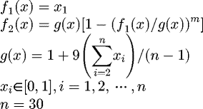 (A.1)
(A.1)
The parameters m = 1/2 and m = 2 correspond to ZDT1 (convex function) and ZDT2 (concave function) respectively. Their ideal Pareto front has been given, as shown by the dotted and dashed lines in Figure A.1. The parameter x1 affects both sub-objective functions and is therefore selected as a characteristic number element. The blue line segments in the figure are the solution intervals obtained by numerical experiments. The number of initial particles corresponding to each numerical experiment is 50, the number of iteration steps is 200, and the total number of experiments is 200. Compared with the ideal Pareto front, it is obvious that the experimental solution converges to the non-inferior optimal solution (PF true) with a certain error range. The average errors of the test solutions of ZDT1 and ZDT2 are e1 = 16.1% and e2 = 11.69%, respectively.
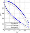 |
Fig. A.1 Ideal Pareto front (PFtrue) and test solution set (EXPERIMENT). |
References
- T.M. Conboy, M.D. Carlson, G.E. Rochau, Dry-cooled supercritical CO2 power for advanced nuclear reactors, J. Eng. Gas Turb. Power 137 , 1 (2015) [Google Scholar]
- V. Dostal, P. Hejzlar, M.J. Driscoll, High-prformance supercritical carbon dioxide cycle for next-generation nuclear reactors, Nucl. Technol. 154, 265–282 (2006) [Google Scholar]
- Y. Ahn, S.J. Bae, M. Kim, S.K. Cho, S. Baik, J.I. Lee, J.E. Cha, Review of supercritical CO2 power cycle technology and current status of research and development, Nucl. Eng. Technol. 47 , 647–661 (2015) [Google Scholar]
- C.S. Turchi, Z.W. Ma, T.W. Neises, M.J. Wagner, Thermodynamic study of advanced supercritical carbon dioxide power cycles for concentrating solar power systems, J. Sol. Energy Eng. Trans. ASME 135 , 7 (2013) [Google Scholar]
- M.A. Reyes-Belmonte, A. Sebastian, M. Romero, J. Gonzalez-Aguilar, Optimization of a recompression supercritical carbon dioxide cycle for an innovative central receiver solar power plant, Energy 112 , 17–27 (2016) [Google Scholar]
- B. Halimi, K.Y. Suh, Computational analysis of supercritical CO2 brayton cycle power conversion system for fusion reactor, Energy Convers. Manag. 63 , 38–43 (2012) [Google Scholar]
- E.M. Clementoni, T.L. Cox, C.P. Sprague, Startup and operation of a supercritical carbon dioxide brayton cycle, J. Eng. Gas. Turb. Power Trans. ASME 136 , 6 (2014) [Google Scholar]
- S.G. Kim, J. Lee, Y. Ahn, J.I. Lee, Y. Addad, B. Ko, CFD investigation of a centrifugal compressor derived from pump technology for supercritical carbon dioxide as a working fluid, J. Supercrit. Fluids 86 , 160–171 (2014) [Google Scholar]
- J.Y. Heo, J. Kwon, J.I. Lee, A study of supercritical carbon dioxide power cycle for concentrating solar power applications using an isothermal compressor, J. Eng. Gas. Turb. Power Trans. ASME 140 , 8 (2018) [Google Scholar]
- Y. Ahn, J. Lee, S.G. Kim, J.I. Lee, J.E. Cha, S.W. Lee, Design consideration of supercritical CO2 power cycle integral experiment loop, Energy 86 , 115–127 (2015) [Google Scholar]
- H. Gurgenci, Supercritical CO2 cycles offer experience curve opportunity to CST in remote area markets, Elsevier Science Bv, Amsterdam, 2014 [Google Scholar]
- E. Drury, G. Brinkman, P. Denholm, R. Margolis, M. Mowers, Exploring large-scale solar deployment in DOE's SunShot vision study, New York, 2012 [Google Scholar]
- C.S. Turchi, Z. Ma, T.W. Neises, M.J. Wagner, Thermodynamic study of advanced supercritical carbon dioxide power cycles for concentrating solar power systems, ASME J. Sol. Energy 135 , 4 (2013) [CrossRef] [Google Scholar]
- W. Zheng, Rotor dynamics design of rotating machinery, Tsinghua University Press, Beijing, 2015 [Google Scholar]
- X.G. Gao Ying, Particle swarm optimization in bionic intelligent computing and its application, Science Press, Beijing, 2018 [Google Scholar]
- V.N. Constantinescu, Gas lubrication, The Research Committee on Lubrication of the ASME, New York, 1969 [Google Scholar]
- L. San Andres, K. Ryu, T.H. Kim, Thermal management and rotordynamic performance of a hot rotor-gas foil bearings system-part I: measurements, J. Eng. Gas. Turb. Power Trans. ASME 133 , 6 (2011) [Google Scholar]
- J.L. Cheng, S. Ronghua, L. Fang, Cognitive computing and multi-objective optimization, Science Press, Beijing, 2017 [Google Scholar]
Cite this article as: J. Li, H. Gurgenci, J. Li, L. Li, Z. Guan, F. Yang, Optimal design to control rotor shaft vibrations and thermal management on a supercritical CO2 microturbine, Mechanics & Industry 22, 22 (2021)
All Tables
All Figures
|
Fig. 1 Supercritical CO2 radial-in-flow turbine lay-out. |
| In the text | |
|
Fig. 2 Approximate rotor shaft geometry. |
| In the text | |
|
Fig. 3 Rotor imbalance response before and after optimization design. |
| In the text | |
|
Fig. 4 SCO2 cooling devices treated in this paper. |
| In the text | |
|
Fig. 5 Dynamic stiffness coefficient versus rotor displacement with different diameters ds. |
| In the text | |
|
Fig. 6 Pressure distributions around an orifice obtained by CFD. |
| In the text | |
|
Fig. 7 Rotor displacement ec versus stiffness kcb. |
| In the text | |
|
Fig. 8 Stiffness coefficient kcb versus mass flow rate Q of the orifice. |
| In the text | |
|
Fig. 9 Three-dimensional finite element model of the rotor system. |
| In the text | |
|
Fig. 10 Verify the effect of the stiffness coefficient of the gas bearing with orifice for ds = 0.12 mm on the synchronous responses of the rotor. |
| In the text | |
|
Fig. 11 The temperature of SCO2 versus free end temperature, calculation condition: (a) din = 2 mm, (b) din = 3 mm, (c) din = 4 mm. |
| In the text | |
|
Fig. 12 Temperature distribution cloud map and gradient comparison chart, din = 4 mm, Hg = 1.5 mm, TCO2 = 350 K, PCO2 = 7 MPa.(a) With hydrostatic zone. (b) No hydrostatic zone. (c) Temperature gradient comparison. |
| In the text | |
|
Fig. 13 Rotor temperature demonstrates that characteristic parameter Hr/din versus cooling efficiency, (a) Given mass flow (q = 0.1 kg/s) of nozzle, (b) Given pressure (1 MPa) of nozzle. |
| In the text | |
|
Fig. A.1 Ideal Pareto front (PFtrue) and test solution set (EXPERIMENT). |
| In the text | |
Current usage metrics show cumulative count of Article Views (full-text article views including HTML views, PDF and ePub downloads, according to the available data) and Abstracts Views on Vision4Press platform.
Data correspond to usage on the plateform after 2015. The current usage metrics is available 48-96 hours after online publication and is updated daily on week days.
Initial download of the metrics may take a while.