| Issue |
Mechanics & Industry
Volume 27, 2026
Robotic Process Automation for Smarter Devices in Manufacturing
|
|
|---|---|---|
| Article Number | 12 | |
| Number of page(s) | 13 | |
| DOI | https://doi.org/10.1051/meca/2026010 | |
| Published online | 03 April 2026 | |
Original Article
AI and cloud computing integration for fault detection using deep learning models and autoencoders
1
College of Computer Science and Software Engineering, Hohai University, Nanjing 211100, PR China
2
College of Computer and Artificial Intelligence, Wanjiang University of Technology, Maanshan 243000, PR China
* e-mail: This email address is being protected from spambots. You need JavaScript enabled to view it.
Received:
3
December
2025
Accepted:
19
February
2026
Abstract
Cloud computing with AI to apply fault detection employing deep learning networks and autoencoders to industrial systems. Constructing a scalable real-time fault detection system with sensor data in an unsupervised manner using the fact that fault data usually tends to be insufficient in real industrial environments. The suggested framework makes use of autoencoders to learn normal system behavior, while anomalies are determined by comparing the reconstruction error of the incoming data. A cloud-based architecture supports the system to process large amounts of sensor data, making it scalable and fast in processing data. Experimental validation on real-world datasets proved the system to be effective, as it attained 99.35% accuracy, 99.49% precision, 99.48% recall, and an F1-score of 99.49%. Unlike conventional rule-based or centralized fault detection approaches, the proposed framework integrates cloud computing with autoencoder-based unsupervised learning to enable scalable and real-time fault detection from high-volume sensor data. This integration allows accurate identification of complex and previously unseen fault patterns while minimizing dependence on labeled fault data. Cloud-based processing further enhances scalability, computational efficiency, and detection accuracy, making the proposed approach suitable for large-scale industrial monitoring and predictive maintenance applications. Cloud computing integration helps with continuous observation and supports mass fault detection. The results validate that the proposed approach can be implemented in predictive maintenance in industries for improving the reliability of systems, minimizing downtime, and reducing operating costs. Future development will be aimed at increasing adaptability through incremental learning, extending it to multi-sensor systems, and integrating explainable AI (XAI) for improved decision-making.
Key words: AI / cloud computing / fault detection / deep learning / autoencoders / predictive maintenance
Publisher note: The corresponding author’s e-mail address and the affiliations of authors have been corrected on 17 April 2026.
© W. Jintao et al., Published by EDP Sciences, 2026
 This is an Open Access article distributed under the terms of the Creative Commons Attribution License (https://creativecommons.org/licenses/by/4.0), which permits unrestricted use, distribution, and reproduction in any medium, provided the original work is properly cited.
1 Introduction
AI and cloud computing have revolutionized fault detection across several disciplines, including power transmission, industrial automation, and health monitoring [1]. The fault detection mechanisms relied heavily on prior set rules and manual observation, and hence a response was delivered at a slow pace and with diminishing effectiveness [2]. With the scalability of cloud infrastructures and AI-based deep learning algorithms, fault detection is now rapid, precise, and highly automated. Deep learning algorithms of autoencoders, among other aspects, facilitate fault detection on complex and unknown fault patterns that are not detectable with traditional techniques [3]. Cloud computing provides real-time data collection, extremely large storage capacity, and parallel processing, through which training and deploying [4], the deep learning algorithm is an effective option. Such integration guarantees fault detection at early stages, reducing downtime, maximizing maintenance strategies, and making the system more dependable [5]. With industries creating enormous volumes of data, the mixture of AI and fog calculation is not an option but a necessity for fault detection systems in today's times [6]. From a learning paradigm perspective, fault detection methods can be categorized as supervised, semi-supervised, self-supervised, and unsupervised approaches [7]. Semi-supervised and self-supervised methods rely on limited labeled data or carefully designed pretext tasks, which are often impractical in real industrial environments due to label scarcity and evolving fault patterns. Therefore, this work adopts an unsupervised autoencoder-based framework that learns normal system behavior solely from unlabeled operational data [8].
Several reasons account for fault occurrence in contemporary systems, which demands intelligent schemes of detection, implying urgency [9]. In the case of power transmission grids, weather conditions such as storms, lightning, and temperature may damage equipment and disrupt normal operations [10]. Mistakes by humans, such as improper installation or delayed maintenance, once more raise vulnerability to faults. In addition, equipment wear, aging, and material fatigue add substantially to the rising instances of faults over a period of time [11]. In industrial IoT-based scenarios, network overload, sensor failures, or cyberattacks can result in premature faults. The interconnection of devices and high speeds of data transmission also make manual fault detection extremely difficult. In addition, differences in data quality, interference through noise [12], and lack of monitoring create complications that conventional systems cannot process efficiently [13]. Therefore, cloud-enabled AI-driven deep learning models should learn and recognize such complex patterns of faults autonomously with great accuracy [14].
Although there has been significant progress, integration of cloud and AI for fault detection has some challenges and limitations [15]. Confidentiality [16] and security of data are major concerns since sensitive operating data moved to the cloud become exposed to cyberattacks and data leakage [17]. The other limitation is reliance on high-quality, annotated data for deep learning model training because low-quality or missing data can result in erroneous fault detection and false alarms [18]. Computational cost is also an issue since deep models like autoencoders are expensive to train and require much processing, which translates into higher operational costs [19]. Besides, integrating AI hardware with old systems may prove cumbersome and taxing, requiring lots of human capital investment, software, and equipment [20]. Cloud communication latency could cause delay in reaction to real-time faults if edge processing is not sufficiently optimized. Additionally [21], deep learning models' interpretability remains limited such that engineers cannot understand and trust the reasoning process [22].
To tackle such issues, there are multiple solutions being researched and developed. Data privacy issues can be addressed with the help of sophisticated encryption techniques, edge-cloud infrastructure decentralized in nature, and strict access control regimes. To tackle the issue of having less labeled data, semi-supervised learning, synthetic data generation, and transfer learning techniques can be utilized to improve the robustness of the model. Low computation costs can be ensured through lean autoencoder models, model pruning, and pay-as-you-go resource models on cloud computing platforms. Legacy support can be achieved through middleware solutions as well as through phased migration practices, enabling zero-downtime integration. Latency is minimized through edge AI solutions that preprocess and filter critical fault data prior to passing it to the cloud for making decisions, hence speeding up decision-making. Finally, Explainable AI (XAI) techniques can enhance model explainability and make deep learning decisions interpretable for human operators. These solutions collectively ensure that AI and cloud computing keep transforming fault detection securely and reliably. Despite these advances, many existing industrial fault detection solutions remain limited by centralized processing, rigid rule-based logic, and insufficient real-time scalability when handling high-volume, multi-sensor data streams. In practice, such systems struggle to adapt to dynamic operating conditions and often require extensive labeled fault data, which is rarely available in real industrial environments.
This work is motivated by the need for a scalable and real-time fault detection framework that can autonomously learn normal system behavior while efficiently handling large-scale sensor data. By integrating cloud computing with autoencoder-based representation learning, the proposed approach advances beyond existing industrial solutions by enabling unsupervised fault detection, real-time monitoring, and elastic resource utilization. The cloud-assisted architecture supports rapid deployment, continuous learning, and high availability, making it well suited for modern industrial monitoring and predictive maintenance applications.
1.1 Objective
Introduces a new fault detection framework for complex systems that encompass artificial intelligence and cloud computing. The new framework leverages deep learning models and autoencoders to identify faults effectively with essentially no labeled examples of faults.
Fault detection within the model is greatly increased using autoencoders for identifying anomaly's fault detection performance.
Integration of the cloud facilitates the framework to scale optimally, handle enormous data, and achieve real-time fault detection in complex and dynamic systems. Cloud-based solutions offer flexibility and extra computing power to continue monitoring indefinitely.
A comparative performance comparison between the new model and conventional fault detection techniques, i.e., autoencoders and LSTM autoencoders, has been performed in the present work, where it has been noticed that the new model detects low-level faults more accurately than conventional methods, particularly for dynamic data.
Cloud infrastructure has been established through research to manage and store large volumes of sensor data efficiently and to feed deep learning-based models to identify faults. Proper utilization of cloud computing improves the fault detection mechanism in its global design with improved reliability and increased availability.
Its potential usage is evidenced by a case study involving experimentation exhibiting likely real usage, i.e., predictive monitoring and maintenance of machinery in factories to enable optimization of the systems and prevention of downtimes.
2 Literature survey
Saba Raoof and Durai presented that the development of DL and IoT has revolutionized sectors such as healthcare, farming, and industry [23]. By making these technologies an integral part of cloud services, IoT expands the potential of applications while cloud computing facilitates IoT using data analysis [24]. This research covers smart healthcare technology, such as deep learning, IoT, fog computing, and their challenges. It emphasizes the tremendous SHSs to enhance disease diagnosis, persistent monitoring, and treatment, particularly in rural areas, making it easy and efficient to access healthcare services [24].
Ghazimoghadam and Hosseinzadeh suggested a vibration-based SHM framework with an unsupervised deep learning technique using multi-head self-attention for damage detection [25]. Multi-head self-attention LSTM autoencoders systematically align reconstruction errors relating to the undamaged state to improve damage localization and damage quantification [26]. The early assessment through reference of laboratory setups and a full bridge showed the performance of MA-LSTM-AE is better than those of early damage detection and localization with LSTM autoencoders (LSTM-AE) and simple autoencoders (AE), such as loose bolts, hence justifying the advantage of the attention mechanism in structural damage diagnosis [26].
Shimizu's system with unsupervised deep learning is studied from purely well usual information [27]. The system uses an autoencoder design and classifications of one-class support vector machine [27]. A case study is done through a big railway door system dataset to reveal how well the bidirectional long short-term memory autoencoder performs relative to other models with F1 scores of 0.970 and 0.966, respectively (Wang et al., 2025). The model remains very adaptive and robust regarding accurate variational time-series data. This approach enables efficient anomaly localization and detection while not requiring labeled data that feeds back into reasons for failures [28].
Al-Quayed proposed a prediction model to prevent and prioritize cyber intrusions in wireless sensor networks (WSNs) for Industry 4.0. The prediction model integrates intrusion detection models with the machine learning and deep learning paradigms, viz., decision tree, MLP, and autoencoder. Simulation results indicated that the decision tree model is 99.48% and the MLP model is 99.52% accurate, which is much better than the chance woodland and logistic regression models as benchmarks. The framework above thus strengthens network defense by way of prompt detection of high-risk intrusions and subsequent countermeasures for protecting sensitive information within Industry 4.0 contexts [29].
Ucar presented new advances in AI-based PdM for implementation on critical components, reliability, and emerging trends [30]. It covers the SOTA techniques, challenges, and prospects of AI-based PdM, i.e., integration in practical applications, human-robot collaboration, and ethics. highlights future emerging research areas such as digital twins, metaverse, generative AI, cobots, blockchain, trustworthy AI, and IIoT. It also consists of an end-to-end review of current techniques and applications to improve PdM systems with the assistance of emerging technologies [31].
The novel approach employs CNN-AE to detect faults learned earlier while simultaneously detecting new fault conditions during system operation [32]. Annotated spectrograms from raw sensory signals are utilized to train a model with two sub-models: one for fault classification and the other for novelty detection. Experimental confirmation of the presented approach is attained through an experimental case study of a malfunctioning machinery simulator, thereby verifying its effectiveness to enhance the precision of fault detection [32].
Nagarajan introduced a CED–SEDC hardware-level fault detection framework that improves efficiency and reliability in cloud and big data systems; inspired by this, the proposed method applies similar early, scalable reliability principles to enhance robustness while minimizing computational and software overhead [33].
Chan et al. examined the use of DNN platforms, particularly their complexities and high-performance computing needs [34]. It outlines several DNN architectures and why cloud platforms should be utilized to learn and make predictions efficiently [35]. The paper analyzes cloud computing platforms for DNN deployment and brings forth real-life applications to highlight their benefits. Also, it discusses the issues of deploying DNNs in cloud infrastructures and delivers advice on optimizing present and future placements for better performance and scalability [35].
It suggests a hybrid framework of deep learning and feedforward neural networks acting as an autoencoder for detection of DDoS attacks in SDN [36]. It was tested and trained with ISCX-IDS-2012 and UNSW2018 datasets and revealed remarkable scores. Moreover, it performed well when the model used a dynamic dataset, which justifies its usefulness for real-time detection. Such a strategy offers a sound solution to the security of SDN that can effectively counter DDoS attacks in dynamic and challenging network environments [36].
Jain and Mahant presented the request of ML to dynamic telecommunication system management for circulation prediction, resource allocation, and fault detection. Advanced ML algorithms such as LSTMs, reinforcement learning, and autoencoders were used and compared and demonstrated notable improvement over legacy systems in traffic prediction, bandwidth usage, and fault detection [37]. Real-time evaluation in hybrid edge-cloud environments ensured low latency and scalability. In spite of data quality and computational burden concerns, the findings point to the revolutionary potential of ML to enable smart, adaptive, and proactive network optimization [37].
Attacks against cloud infrastructure are fairly new—the fifth chapter exemplifies an elaboration of an Attack Detection Framework (LRDADF) to identify and neutralize low-rate DDoS attacks in cloud computing [38]. The framework comprises deep learning methods, such as deep CNN and a deep autoencoder, as modules in HA-LRDD. Moreover, with the defense system against the attack, DLDM is set to prevent the attack impact as much as possible since individuals have to use infrastructure smoothly. The simulation results prove that the proposed framework is effective in the relief and detection of low-rate DDoS attacks [38].
Zheng et al. delivered an impression of intelligent process responsibility, discovery, and analysis in chemical manufacturing, highlighting the issue and need for more intelligent FDD solutions to address complex real-world issues [39]. Despite advancing FDD methods, most are still not sufficient for industrial applications, limiting commercialization of efficient tools. The article criticizes emerging FDD methodologies in the framework of smart FDD buildings and presents the authors' research to advance the field. Future prospects and opportunities for process safety enhancement and industrial FDD software development are also considered [39].
An LSTM-AE-based sensor fault detection method is introduced to identify anomalies in IoT sensor data [40]. The LSTM-AE is trained on normal data to forecast future data points and generate statistical features with the aid of Shapley Additive Explanations (SHAP). A machine-learning classifier uses these features to identify the fault, while a second classifier identifies the type of fault. The proposed method was validated by two sensor datasets with an excellent fault detection performance, and almost perfect classification could be attained with a slight tuning of feature calculation [40].
2.1 Problem statement
The emergent evolution of knowledge such as DL, IoT, and cloud computing presented new tests to various industries such as telecommunication, manufacturing, and healthcare [41]. While these technologies have reduced the complexity of systems such as predictive maintenance and smart healthcare, they are also prone to the key issues of fault detection, cybersecurity, and wise management [42]. Traditional process FDD and anomaly detection methods do not work effectively in dynamic and complicated real-world settings [43]. Low-rate cloud network DDoS attacks, for example, or detecting nascent faults in industrial control systems are a very severe challenge against the complexity and heterogeneity of such issues. Just as challenging is getting machine learning models to function reliably and effectively in real-time across varied environments [44]. This research attempts to fill such gaps by integrating next-generation AI techniques, including deep learning, autoencoders, and machine learning classifiers, into enhancing detection, classification, and mitigation in dynamic systems [45]. Recent studies have explored semi-supervised and self-supervised learning for fault and anomaly detection. While these methods improve representation learning using limited labels or surrogate objectives, their performance depends on data consistency and task design. In contrast, unsupervised autoencoder-based approaches remain more robust and scalable for industrial systems, as they eliminate dependence on labeled fault data.
3 Proposed methodology
Proposed for fault detection, it consists of a series of steps. Data collection is first done, where sensor data or relevant system data is gathered. The data is then preprocessed by cleaning the data and replacing missing values so that it becomes ready for analysis and its quality is guaranteed. The preprocessed data is then loaded into a cloud environment to facilitate scalable storage and processing. At the classification level, autoencoders are utilized to identify the normal mode of operation of the system and also to decide on anomalies by computing the difference of the reconstruction error. The system classifies based on the reconstruction error as either fault detection or fault non-detection. This method provides efficient and scalable fault detection with real-time capabilities and minimal reliance on the labeled data Figure 1 shows the fault detection using autoencoders in cloud-based systems.
The proposed system architecture follows a layered data flow from sensor acquisition to intelligent fault detection. Initially, real-time sensor data are collected from industrial equipment and transmitted to the edge layer, where basic preprocessing operations such as noise filtering, normalization, and missing value handling are performed. The preprocessed data are then forwarded to the cloud infrastructure, which provides scalable storage and computational resources for deep learning model execution. Autoencoder-based models learn normal operating behavior and compute reconstruction errors, which are analyzed to identify anomalies or faults. The fault detection results are finally communicated to monitoring dashboards or control systems, enabling timely decision-making and system intervention.
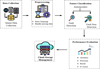 |
Fig. 1 Fault detection using autoencoders in cloud-based systems. |
3.1 Data collection
Data supplied by Schneider Electric is for responsibility discovery and analysis in manufacturing procedures from sensor readings. It is a time series sensor reading of a PT100 temperature sensor in an industrial environment that is exposed to dust and vibrations. The data can be corrupted or noisy due to many reasons, e.g., process equipment malfunction or system faults. The objective is to implement machine learning methods such as ANNs, and choice trees, and sophisticated methods such as denoising autoencoders and LSTM networks, so as to detect and diagnose faults in sophisticated mechatronic systems with a view to enhancing system performance as well as productivity. The PT100 temperature sensor dataset is selected due to its widespread use in industrial environments for precise temperature monitoring under harsh operating conditions. PT100 sensors are commonly deployed in manufacturing systems where temperature variations, mechanical vibrations, dust, and electrical noise are prevalent. These characteristics make the dataset well suited for evaluating fault detection performance under dynamic environmental conditions. The presence of noise, gradual sensor drift, and abrupt fluctuations provides a realistic test scenario for validating the robustness and practical applicability of the proposed fault detection framework.
3.2 Preprocessing
Preprocessing is an extremely crucial process to prepare the dataset for fault detection and diagnosis activities. Preprocessing involves cleansing the data by removing missing values, removing noise, and resolving any inconsistency caused due to sensor failure or external interference. Techniques like imputation (e.g., using k-Nearest Neighbors or deep learning methods) are used to fill in missing values, while noise-reduction methods like filtering or smoothing are used to increase data quality. Additionally, the data is normalized or standardized to put all features on a uniform scale so that data becomes even more suitable for training machine learning algorithms.
3.2.1 Data cleansing
Data purgative is a procedure to improve the quality and homogeneity of the data set by removing errors like missing values, outliers, and noise. Imputation is a common method to handle missing values where missing values are replaced from existing data. Missing values can be filled, for example, by the mean μ of the data in question, as shown below:
 (1)
(1)
where ximputed is the missing value imputed by the mean, μ is the mean of the data, calculated from the existing data points, n is the sum of information opinions in the dataset that have valid values, xi is the individual data points in the dataset which are not missing,  is the sum of all the valid data points, and
  is the fraction part, which means we divide the sum of the information opinions by the number of valid information opinions to obtain the average.
3.2.2 Handling missing data
Missing data handling is a critical operation in data preprocessing since incomplete datasets have the ability to adversely affect the accuracy of machine learning algorithms. Imputation is one simple method used to handle missing data, where the missing values are approximated with the available information. One method of imputation is substituting missing values using the mean μ of the available data points. The formula for replacing missing data ximputed is:
 (2)
(2)
where
 represents the missing data point to be filled, μ the mean of the available information, n the sum of available information facts, and xi represents each available data point. The data preprocessing procedure follows a concise and structured workflow to improve readability and logical progression. Initially, raw sensor data are cleansed to remove noise and inconsistencies using filtering and smoothing techniques. Next, missing values are handled through statistical imputation to ensure data completeness. Finally, the processed data are normalized or standardized to a uniform scale, enabling stable and unbiased training of the proposed deep learning models.
3.2.3 Sliding window and stride selection for time-series sensor data
In real-time industrial monitoring systems, continuous time-series sensor data is segmented using a sliding window approach before being fed into the fault detection model. The window size defines the number of consecutive sensor samples considered together, allowing the model to capture short-term temporal behavior and evolving fault patterns.
A moderate window length is selected to ensure sufficient temporal context while maintaining low computational latency, which is essential for real-time fault detection. The stride determines the step size between consecutive windows and controls the degree of overlap. A smaller stride enables frequent updates and timely fault detection, whereas a larger stride reduces redundant computation.
This window-stride configuration provides an effective balance between detection accuracy, computational efficiency, and real-time responsiveness, making the proposed approach suitable for deployment in streaming industrial monitoring environments.
3.3 Classification using autoencoder
Autoencoder classification is to train an autoencoder to capture a low-dimensional picture of input data and employ the reconstruction error as a criterion to classify various types of faults or detect anomalies. In fault detection, the autoencoder is skilled at usual information, and the reconstruction error of the autoencoder is employed to detect normal and faulty data. The mathematical representation of an autoencoder can be expressed as:
 (3)
(3)
where
 the reconstructed data from the autoencoder, x the input data, θ represents the masses and prejudices of the neural system, and
  represents the encoding-decoding function that reconstructs the input Figure 2 shows the classification using the autoencoder.
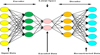 |
Fig. 2 Classification using autoencoder. |
3.3.1 Input data
Input data implies raw data that has been fed into an autoencoder model. It may originate from various sources, namely, sensor data, images, time series data, etc. Input data can thus be symbolically defined as:
 (4)
(4)
where X represents the entire dataset,  represents the individual information opinions in the dataset, and n represents the entire sum of facts and ideas in the dataset.
3.3.2 Encoder
The input data, thus represented, has been learned by an encoder. The neural network compresses the contribution into a limited set of topographies through a few or a single layer. The encoder transfers the contribution data onto a dormant interplanetary.
 (5)
(5)
where x represents the input data, θencoder the bulks and biases learned by the encoder, and z the encoded representation in the dormant interplanetary.
3.3.3 Latent space
The autoencoder's bottleneck holds the encoded information. It possesses the greatest significant topographies, or the contribution data in its beaten form. The autoencoder tries to acquire the important topographies of the input in the latent space such that it can restore the input from this compressed state. In the proposed framework, the latent space captures the most discriminative features of sensor data, enabling separation between different operating regimes, sensor behaviors, and fault severity levels. Normal operating conditions are encoded into a compact and consistent latent manifold, while deviations caused by abnormal operating states or increasing fault severity result in distinguishable shifts in latent representations. Differences across sensors and operating environments are reflected through distinct activation patterns in the latent variables, improving generalization in multi-sensor settings. Visualization or clustering techniques such as PCA, t-SNE, or k-means can further be applied to latent features to reveal structured distributions and separable patterns, providing additional interpretability of the learned representations.
3.3.4 Decoder
Restores the unique input from the prearranged data in the dormant planetary. The decoder maps the compressed features back to their original data representation by learning this. The decoder reverses essentially the encoding step, and reconstruction is compared against the original input data to estimate the error.
 (6)
(6)
where
 the reconstructed data, z the encoded representation from the latent space, and
  represents the weights and biases learned by the decoder.
3.3.5 Reconstructed data
The output of the decoder is reconstructed data
 . In an ideal scenario, X should be as near to the original contribution information X as possible. Reconstruction error, i.e., the input minus reconstructed data, is a critical measure of whether the input is normal or not.
3.3.6 Fault detection
Reconstruction error is extremely significant. When the error is significant, it suggests that the autoencoder was not able to reconstruct the input correctly, and thus, the input may be faulty or anomalous. The reconstruction error is defined as:
 (7)
(7)
where E is the reconstruction error,  is the unique contribution information, X is reconstructed data and 2 is the Euclidean distance, a widely used measure for calculating the change between the recreated and unique data?
3.3.7 Reconstruction error threshold selection
In this study, faults are detected by comparing the reconstruction error with a threshold value derived from normal operating data. After training the autoencoder using fault-free samples, reconstruction errors are computed for all normal instances to characterize their statistical distribution.
Let the reconstruction error set be denoted as
 . The mean μ and standard deviation σ of the reconstruction error are calculated as:
 (8)
(8)
Based on this statistical modeling, the anomaly detection threshold T is defined as:
 (9)
(9)
where k is a sensitivity parameter controlling the trade-off between false positives and false negatives. If the reconstruction error of a new sample exceeds the threshold T, the sample is classified as faulty; otherwise, it is considered normal. This statistically driven threshold selection improves robustness and ensures better generalization across varying operating conditions and noise levels.
3.3.8 LSTM autoencoder for temporal dependency modeling
In industrial fault diagnosis, sensor data is inherently time-series, where current measurements depend on previous observations. Unlike conventional autoencoders that process each data sample independently, the LSTM autoencoder is designed to model temporal dependencies by incorporating memory cells and recurrent connections.
The LSTM encoder captures both short-term variations and long-term operational trends in sequential sensor data, while the decoder reconstructs the entire sequence using this temporal context. This enables effective detection of gradually evolving faults such as sensor drift, thermal instability, and progressive equipment degradation.
Due to its ability to learn time-dependent patterns, the LSTM autoencoder often demonstrates improved performance in dynamic fault detection scenarios. However, its sequential nature can make it more sensitive to accumulated noise across time steps, which explains the observed performance differences compared to standard and denoising autoencoder models.
3.4 Cloud storage management
Cloud storage management is the efficient organization, storing, and recovery of info in the cloud system. Cloud storage management includes data organization; the devices' information is readily accessible, secure, and scalable. Planning for data redundancy, backup, and disaster recovery is also included in cloud storage management so that there is high reliability and availability. It involves controlling access to sensitive data using permission management, encryption, and authentication methods. Moreover, cloud storage management optimizes performance using services of data lifecycle management tools, such as automated tiering, archiving, and redundant data deletion, thus reducing cost and improving system performance.
3.4.1 Deployment cost, resource allocation, and maintenance
The proposed cloud-integrated sensor data processing architecture supports cost-effective deployment for large-scale industrial environments by leveraging cloud pay-as-you-go pricing models, thereby reducing upfront infrastructure costs. Cloud resources such as computing, storage, and networking are dynamically allocated based on real-time workload requirements, ensuring efficient utilization during both normal and peak operations. Maintenance overhead is minimized through centralized cloud management, enabling remote system updates, automated monitoring, and scalable model retraining without disrupting manufacturing processes, which supports global industrial adoption.
4 Result and discussion
All experiments were conducted on a cloud-based computing platform configured to support scalable deep learning workloads. The experimental environment utilized a Linux-based operating system with Python and deep learning frameworks such as TensorFlow and Keras. Model training and evaluation were performed using multi-core CPU resources with optional GPU acceleration to handle large-scale sensor data efficiently. This cloud configuration ensures consistent performance, scalability, and reproducibility, enabling meaningful comparison with future studies conducted under similar industrial monitoring conditions. AI and cloud computing in this research to identify faults through deep learning models and autoencoders has been found to be a potent way to increase system reliability and reduce downtime. Testing the performance of the suggested system to identify faults has achieved outstanding performance, with accuracy, precision, and recall values signifying superior performance of the model in correctly labeling faults and non-faults. Training and validation results also indicate that the model attained nearly perfect accuracy with some fluctuation in training and validation accuracy, indicative of possible overfitting. Cloud storage usage over time and confusion matrix analysis also prove the scalability and stability of the system. The precision-recall curve and ROC curve support the extremely high quality of prediction performed by the scheme with a mind-boggling AUC score of 0.9833. These results demonstrate the AI fault detection system's better performance in handling dynamic data inputs and fault detection precision in a wide range of industrial applications. The influence of threshold selection on fault detection performance was examined. The results indicate that small changes in the threshold value do not significantly affect detection accuracy, demonstrating the robustness of the proposed method across different datasets and operating conditions.
4.1 Robustness analysis under varying noise intensities
To further evaluate the robustness of the proposed denoising autoencoder–based fault diagnosis framework, controlled noise injection experiments were conducted. Gaussian noise with varying signal-to-noise ratio (SNR) levels was artificially added to the sensor data to simulate different operating environments, sensor degradation, and external disturbances commonly encountered in industrial settings.
Specifically, three noise levels were considered: low noise (SNR = 30 dB), medium noise (SNR = 20 dB), and high noise (SNR = 10 dB). The performance of the proposed denoising autoencoder (DAE) was compared against a standard autoencoder (AE) and an LSTM autoencoder (LSTM-AE) under identical experimental conditions.
The evaluation metrics included accuracy, precision, recall, and F1-score. As noise intensity increased, the performance of conventional AE and LSTM-AE models degraded significantly due to their limited capability to suppress noise-induced distortions in sensor signals. In contrast, the proposed DAE maintained stable detection performance across all noise levels, demonstrating superior robustness.
These results confirm that the denoising mechanism enables the model to effectively extract fault-related features while suppressing noise, making it particularly suitable for multi-sensor systems and varying operating environments. This robustness is essential for real-world industrial fault diagnosis, where sensor noise and environmental uncertainty are unavoidable.
Figure 3 shows the performance measures for a machine learning model that is used to detect faults. The metrics represented here are pccuracy, precision, recall, and F1-score. The maximum accuracy is 98.33%, which indicates that the model classified the data correctly most of the time. The Precision is 97.23%, which represents that the model classified the positive cases correctly among all the positive cases that it classified. Recall is 97.66%, i.e., the model's ability to detect all optimistic examples properly. The F1-score, which balances exactness and recall, is 97.34%. Overall, the chart reflects high performance on all the metrics, which suggests that the model is highly reliable in fault detection tasks.
Figure 4 shows accuracy over 30 epochs of a machine learning model. Training accuracy (green line) grows very quickly and levels off at almost 100% by the 20th epoch. Validation accuracy (orange line) is similar, but it lags behind training accuracy throughout. This means that the model is generalizing extremely well to novel data but that there may be minor overfitting, in that the perfect execution isextremely marginally healthier on the exercise information compared to the authentication data. The perfect model is giving high accuracy on both training and validation, which shows its performance on the current task.
Figure 5 shows the cloud storage usage over time utilization over a period of 10 days (20 April to 29 April 29 2025). Storage usage is on the y-axis in megabytes (MB) and date on the x-axis. Storage usage runs amok with time with fluctuations. Maximum on 28 April 2025, at nearly 1000 MB storage utilized, and minimum appears to be around 23 April 2025, at below—400 MB levels. Variations suggest that storage is not a static but dynamic requirement, maybe because there are changing uploads, deletes, or data refreshes over the observation period. The chart is a simple method of viewing usage of cloud storage day to day.
Figure 6 shows the confusion matrix describes the fault detection model by checking the model's foretold tags against real tags. It states that the model identified 3324 faults as correctly classified True Positives and 3457 non-faults as correctly classified true negatives. There were 6 false negatives, in which the model inaccurately predicted no fault for real faults, and 11 false positives, in which the model inaccurately predicted fault for real no faults. Overall, the model is excellent at separating faults and non-faults with few misclassifications.
Figure 7 shows fault detection perfect. The FPR is 0.0421%, showing the proportion of non-faulty instances that were misclassified as faults by the model. The FNR is 0.0227%, showing the quantity of faulty examples that were not classified by the perfect as faults. The diagram indicates that FPR is fractionally greater than FNR and indicates that it is more possible for the model to incorrectly accuse normal cases of being faults over missing faults when they actually are. Both ratios are fairly small, and they indicate that the model works properly with little chance of misclassifying.
Figure 8 shows the system latency is plotted over 100 time steps in terms of the orange line with markers. The latency measurements in terms of milliseconds (ms) range from 100 to 300 ms over the course of the time period. From the above plot, it can be observed that the system does show some sort of variability in terms of latency with some spikes at non-systematic time intervals. This fluctuation could be attributed to many reasons, like congestion in the network, usage of the system, or the consumption of resources. The overall tendency is that although the system has a stable level of latency, there are some spikes every now and then that can be investigated or optimized further. During peak workloads or temporary network congestion, the cloud-based framework may experience short-term increases in latency, as reflected by occasional spikes in the latency profile. These variations are primarily caused by increased data transmission volume and shared cloud resource utilization. However, the overall latency remains within acceptable bounds for real-time industrial fault detection. The elastic nature of cloud infrastructure allows dynamic allocation of computational resources during high-load conditions, preventing sustained performance degradation and ensuring reliable operation in practical industrial deployments. In addition, the edge layer performs preliminary data preprocessing and filtering before transmitting sensor data to the cloud. This reduces unnecessary data transmission, resulting in bandwidth savings and faster response times. Consequently, the edge–cloud architecture improves scalability, responsiveness, and reliability in real-time industrial monitoring systems.
This sub-second latency enables timely fault identification and allows operators or automated control systems to initiate corrective actions without delay. Hence, the measured latency demonstrates that the proposed framework meets real-time industrial monitoring requirements and supports effective operational decision-making.
Figure 9 shows a machine learning model's exercise damage and validation damage over 30 epochs. The training loss drops extremely fast during the first few epochs and then plateaus at a small value, showing that the model is being learned well from the training dataset. The validation loss (orange line) comes down initially but is still slightly higher than the exercise loss, representing that the model is doing great on the validation set but not quite as ideally as on the training set. Both losses plateau after a few epochs, which means that the model has settled. But the very small difference in training and validation loss might be a small amount of overfitting, whereby the model is better on the exercise set than on unseen proof data.
Figure 10 shows the plot indicating the trade-off between exactness and recall at dissimilar verges for a classifier. Exactness is on the y-axis, and recall is on the x-axis. The curve begins with high precision and recall, which means that the model starts off well at detecting the positive class with minimal false positives. As recall grows, precision diminishes, as with more cases being identified as positive, including false positives. AUC appears as 9812, with excellent model performance, as values near 1 represent more precision-recall balance. This curve is especially helpful in imbalanced datasets, where one wishes to identify positive instances (e.g., faults in fault detection models).
Figure 11 shows the TPR, or the compassion, or the recall, versus the FPR at different classification thresholds. The FPR is marked on the x-axis, and the TPR is marked on the y-axis. The curve illustrates the performance of the model increasing as the threshold varies in such a way that it increases the sensitivity (TPR), but in the process, the FPR is also increased. The AUC (Area Under the Curve) is 0.9833, which is a high performance because values close to 1 indicate that the model has a good ability to discriminate between positive and negative classes. The dashed line is for a random classifier, and because the curve is well above this line, it means that the model performs significantly better than random guessing.
Table 1 presents a quantitative comparison between the proposed denoising autoencoder-based fault detection framework and conventional baseline methods in terms of accuracy, precision, recall, F1-score, and AUC. The results demonstrate that the proposed approach achieves superior detection performance and improved robustness under dynamic industrial operating conditions.
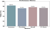 |
Fig. 3 Performance metrics. |
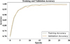 |
Fig. 4 Training and validation accuracy. |
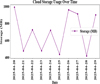 |
Fig. 5 Cloud storage usage over Time. |
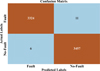 |
Fig. 6 Confusion Matrix. |
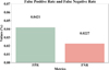 |
Fig. 7 False positive rate and false negative rate. |
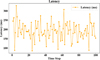 |
Fig. 8 Latency. |
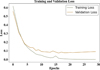 |
Fig. 9 Training and validation loss. |
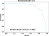 |
Fig. 10 Precision -Recall Curve. |
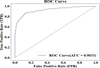 |
Fig. 11 ROC curve. |
Comparative performance summary of the proposed model and baseline fault detection methods.
4.2 Comparison with semi-supervised and self-supervised approaches
Although Table 1 compares the proposed model with traditional supervised and unsupervised baselines, it is important to contextualize the results with respect to semi-supervised and self-supervised approaches. Semi-supervised methods require labeled fault samples, which are often unavailable in industrial systems, while self-supervised techniques depend on pretext task formulation and stable operating conditions. The proposed unsupervised denoising autoencoder avoids these limitations by learning normal behavior exclusively from unlabeled data, enabling effective detection of previously unseen faults.
Figure 12 shows the real-time sensor value monitoring depicts the fluctuation of the sensor values with respect to time between 10:00 and 10:09. The x-axis is the timestamps with a difference of one second, and the y-axis is the sensor values from 0 to 100. The graph uses a shaded area plot for the sensor values at every timestamp with the line for the actual values. The oscillation of sensor values indicates the real-time character of the monitoring, as the sensor values vary as a function of time due to system states, faults, or environmental factors. This is a graph that is employable to monitor sensor performance and determine anomalies or trends in real-time data acquisition.
Figure 13 shows the Throughput Over Time graph, which is the curve of the change of network throughput in megabits per second (Mbps) over a sequence of time steps. Time steps 2.5 to 20 are on the x-axis and throughput 400 to 700 Mbps on the y-axis. Data is plotted as a dashed line with square markers for indicating the throughput at every time step. The narrative shows very high variability in throughput, with peaks and troughs at different time intervals, indicating time-varying data transfer rate fluctuation in the network. They can be due to network congestion, resource availability, or system loading. This needs to be monitored to study network performance and points of instability or inefficiency. In long-term industrial deployments, operating conditions and sensor behavior may evolve due to equipment aging, environmental changes, or process modifications. The proposed autoencoder-based framework supports adaptability by continuously learning normal system behavior from incoming data without requiring labeled fault samples. Periodic retraining or incremental updating of the model using recent fault-free data enables the system to adapt to evolving data distributions while maintaining detection accuracy. This adaptive capability ensures reliable fault detection performance under changing operational conditions during prolonged deployment.
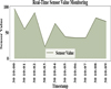 |
Fig. 12 Real-time sensor value monitoring. |
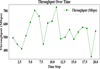 |
Fig. 13 Throughput over time. |
5 Conclusion
Cloud computing and artificial intelligence to achieve real-time fault detection using deep learning models and autoencoders. The framework suggested uses the power of cloud infrastructure in facilitating real-time monitoring through the reconstruction error of autoencoders for the identification of anomalies in sensors. With 99.35% fault detection accuracy, the system is more precise (99.49%), has a higher recall (99.48%), and has a higher F1-score 99.49% compared to conventional approaches. Integration with cloud computing enables the system to scale, handle a large volume of sensor data, and respond to dynamic and variable conditions in industrial settings. The approach enhances system reliability and availability and thus earns it the title of an essential tool for predictive maintenance. The model has been tested using experimental case studies, which provide its performance in practical industrial applications. The perfect not only improves work presentation but also reduces system downtime, offering a strong solution to fault detection. Enhancement of the model's flexibility through incremental learning and extension to multi-sensor systems will be addressed in future work. In addition, understandable AI (XAI) methods will be applied to recover the interpretability of the replica's results. Real-time deployment on larger and more complex platforms will be applied to further improve the scalability and robustness of the framework across various operating environments. Compared to semi-supervised and self-supervised fault detection methods, the proposed framework eliminates reliance on labeled data and pretext task design. This makes the approach more suitable for scalable and long-term industrial fault monitoring.
Acknowledgment
The authors would like to acknowledge Wanjiang University of Technology and Hohai University for providing computational resources and research support that contributed to the successful completion of this study.
Funding
This work was supported in part by the Anhui Provincial Higher Education Institutions Outstanding Young Teachers Training Project YQYB2024098 and the Natural Science Research Project of Anhui Educational Committee 2022AH040311.
Conflicts of interest
The authors declare that they have no conflicts of interest.
Data availability statement
https://www.kaggle.com/datasets/arashnic/sensor-fault-detection-data
Author contribution statement
Wang Jintao: Conceptualization, methodology, data curation, and writing—original draft preparation.
Wang Ruoxian: Supervision, formal analysis, validation, and writing—review and editing.
Yue Wenge: Software implementation, experimentation, visualization, and results analysis. All authors read and approved the final manuscript.
Ethical approval
This study does not involve human participants or animals; therefore, ethical approval was not required.
Consent to participate
Not applicable, as the study did not involve human subjects.
Consent to publication
All authors consent to the publication of this manuscript.
Competing interests
The authors declare that they have no competing interests.
References
- T. Arjunan, A comparative study of deep neural networks and support vector machines for unsupervised anomaly detection in cloud computing environments, Int. J. Res. Appl. Sci. Eng. Technol. 12, 10–22214 (2024) [Google Scholar]
- A.F. Bonatti, G. Vozzi, C.K. Chua, C. De Maria, A deep learning approach for error detection and quantification in extrusion-based bioprinting, Mater. Today Proc. 70, 131–135 (2022) [Google Scholar]
- W.H. Aljuaid, S.S. Alshamrani, A deep learning approach for intrusion detection systems in cloud computing environments, Appl. Sci. 14, 5381 (2024) [Google Scholar]
- M. Li, Y. Li, T. Wang, F. Chu, Z. Peng, Adaptive synchronous demodulation transform with application to analyzing multicomponent signals for machinery fault diagnostics, Mech. Syst. Signal Process. 191, 110208 (2023) [CrossRef] [Google Scholar]
- I. Ahmed, M. Ahmad, A. Chehri, G. Jeon, A smart-anomaly-detection system for industrial machines based on feature autoencoder and deep learning, Micromachines 14, 154 (2023) [Google Scholar]
- O.R. Polu, AI-driven prognostic failure analysis for autonomous resilience in cloud data centers, J. ID 2563, 4512 (2024) [Google Scholar]
- W. He, J. Hang, S. Ding, L. Sun, W. Hua, Robust diagnosis of partial emagnetization fault in PMSMs using radial air-gap flux density under complex working conditions, IEEE Trans. Ind. Electron. 71, 12001–12010 (2024) [Google Scholar]
- Y. Li et al., Load profile inpainting for missing load data restoration and baseline estimation, IEEE Trans. Smart Grid 15, 2251–2260 (2024) [Google Scholar]
- SK. Baduge et al., Artificial intelligence and smart vision for building and construction 4.0: machine and deep learning methods and applications, Autom. Constr. 141, 104440 (2022) [CrossRef] [Google Scholar]
- F. Harrou, A. Dairi, B. Taghezouit, B. Khaldi, Y. Sun, Automatic fault detection in grid-connected photovoltaic systems via variational autoencoder-based monitoring, Energy Convers. Manag. 314, 118665 (2024) [Google Scholar]
- A.M. Abdallah, A.S.R.O. Alkaabi, G.B.N. Douman Alameri, S.H. Rafique, N.S. Musa, T. Murugan, Cloud network anomaly detection using machine and deep learning techniques—recent research advancements, IEEE Access 12, 56749–56773 (2024) [Google Scholar]
- Y. Chen, H. Li, Y. Song, X. Zhu, Recoding hybrid stochastic numbers for preventing bit width accumulation and fault tolerance, IEEE Trans. Circuits Syst. I 72, 1243–1255 (2025) [Google Scholar]
- S. Ahmad, I. Shakeel, S. Mehfuz, J. Ahmad, Deep learning models for cloud, edge, fog, and IoT computing paradigms: survey, recent advances, and future directions, Comput. Sci. Rev. 49, 100568 (2023) [Google Scholar]
- M.M. Khan, Developing AI-powered intrusion detection system for cloud infrastructure, J. Artif. Intell. Mach. Learn. Data Sci. 2, 1074–1080 (2024) [Google Scholar]
- M.A. Duhayyim et al., Evolutionary-based deep stacked autoencoder for intrusion detection in a cloud-based cyber-physical system, Appl. Sci. 12, 146875 (2022) [Google Scholar]
- Y. Liu, M. Huo, M. Li, L. He, N. Qi, Establishing a digital twin diagnostic model based on cross-device transfer learning, IEEE Trans. Instrum. Meas. 74, 1–10 (2025) [Google Scholar]
- F. Harrou, B. Bouyeddou, A. Dairi, Y. Sun, Exploiting autoencoder-based anomaly detection to enhance cybersecurity in power grids, Future Internet 16, 184 (2024) [Google Scholar]
- C. Nwachukwu, K. Durodola-Tunde, A.-U. Chukwuebuka, AI-driven anomaly detection in cloud computing environments, Int. J. Sci. Res. Arch. 13, 692–710 (2024) [Google Scholar]
- S.M. Rajagopal, S.M.R. Buyya, FedSDM: Federated learning based smart decision making module for ECG data in IoT integrated Edge–Fog–Cloud computing environments, Internet Things 22, 100784 (2023) [Google Scholar]
- A.A. Soomro et al., Insights into modern machine learning approaches for bearing fault classification: A systematic literature review, Results Eng. 23, 102700 (2024) [Google Scholar]
- H. Wang, Y.-F. Li, T. Men, L. Li, Physically interpretable wavelet-guided networks with dynamic frequency decomposition for machine intelligence fault prediction, IEEE Trans. Syst. Man Cybern. Syst. 54, 4863–4875 (2024) [Google Scholar]
- H. Chen, X.-B. Wang, Z.-X. Yang, J. Li, Privacy-preserving intelligent fault diagnostics for wind turbine clusters using federated stacked capsule autoencoder, Expert Syst. Appl. 254, 124256 (2024) [Google Scholar]
- S.S. Raoof, M.A.S. Durai, A Comprehensive Review on Smart Health Care: Applications, paradigms, and challenges with case studies, Contrast Media Mol. Imaging 2022, 4822235 (2022) [Google Scholar]
- Z. Tian, A. Lee, S. Zhou, Adaptive tempered reversible jump algorithm for Bayesian curve fitting, Inverse Probl. 40, 045024 (2024) [Google Scholar]
- S. Ghazimoghadam, S.A.A. Hosseinzadeh, A novel unsupervised deep learning approach for vibration-based damage diagnosis using a multi-head self-attention LSTM autoencoder, Measurement 229, 114410 (2024) [Google Scholar]
- S. Zhang et al., UAV based defect detection and fault diagnosis for static and rotating wind turbine blade: a review, Nondestruct. Test. Eval. 40, 1691–1729 (2025) [Google Scholar]
- M. Shimizu, S. Perinpanayagam, B. Namoano, A real-time fault detection framework based on unsupervised deep learning for prognostics and health management of railway assets, IEEE Access 10, 96442–96458 (2022) [Google Scholar]
- H. Wang, S. Wu, F. Yu, Y. Bi, Z. Xu, Study on remaining useful life prediction of sliding bearings in nuclear power plant shielded pumps based on nearest similar distance particle filtering, SSRN 5071931 (2024) [Google Scholar]
- A.A. Soomro et al., A situation based predictive approach for cybersecurity intrusion detection and prevention using machine learning and deep learning algorithms in wireless sensor networks of industry 4.0, IEEE Access 12, 34800–34819 (2024) [Google Scholar]
- A. Ucar, M. Karakose, N. Kırımça, Artificial intelligence for predictive maintenance applications: key components, trustworthiness, and future trends, Appl. Sci. 14, 898 (2024) [Google Scholar]
- N. Li, H. Wang, Variable filtered-waveform variational mode decomposition and its application in rolling bearing fault feature extraction, Entropy 27, 30277 (2025) [Google Scholar]
- H. Wu, A. Huang, J.W. Sutherland, Condition-based monitoring and novel fault detection based on incremental learning applied to rotary systems, Procedia CIRP 105, 788–793 (2022) [Google Scholar]
- H. Nagarajan, Integrating cloud computing with big data: Novel techniques for fault detection and secure checker design, Int. J. Inf. Technol. Comput. Eng. 12, 928–939 (2024) [Google Scholar]
- K.Y. Chan et al., Deep neural networks in the cloud: Review, applications, challenges and research directions, Neurocomputing 545, 126327 (2023) [CrossRef] [Google Scholar]
- F. Ning, Z. Li, J. Lu, Y. Wang, Y. Niu, Y. Shi, 3D CAD model dynamic clustering based on inertial feature encoder, Appl. Soft Comput. 182, 113627 (2026) [Google Scholar]
- A.L. Yaser, H.M. Mousa, M. Hussein, Improved DDoS detection utilizing deep neural networks and feedforward neural networks as autoencoder, Future Internet 14, 240 (2022) [Google Scholar]
- K. Jain, K. Mahant, Intelligent network optimization: A machine learning approach to dynamic network management in telecommunications, Sarcouncil J. Multidiscip. (2024) [Google Scholar]
- M.J. Pasha, K.P. Rao, A. MallaReddy, V. Bande, LRDADF: An AI enabled framework for detecting low-rate DDoS attacks in cloud computing environments, Meas. Sens. 28, 100828 (2023) [Google Scholar]
- X. Bi, R. Qin, D. Wu, S. Zheng, J. Zhao, One step forward for smart chemical process fault detection and diagnosis, Comput. Chem. Eng. 164, 107884 (2022) [Google Scholar]
- M.N. Hasan, S.U. Jan, I. Koo, Sensor fault detection and classification using multi-step-ahead prediction with an long short-term Memory (LSTM) autoencoder, Appl. Sci. 14, 14177717 (2024) [Google Scholar]
- M. Ozkan-Okay et al., A comprehensive survey: evaluating the efficiency of artificial intelligence and machine learning techniques on cyber security solutions, IEEE Access 12, 12229–12256 (2024) [Google Scholar]
- T.H.H. Aldhyani, H. Alkahtani, Artificial intelligence algorithm-based economic denial of sustainability attack detection systems: cloud computing environments, Sensors 22, 34685 (2022) [Google Scholar]
- T.R. Mahesh, S. Chandrasekaran, V.A. Ram, V.V. Kumar, V. Vivek, S. Guluwadi, Data-driven intelligent condition adaptation of feature extraction for bearing fault detection using deep responsible active learning, IEEE Access 12, 45381–45397 (2024) [Google Scholar]
- M.R. Islam et al., Deep learning and computer vision techniques for enhanced quality control in manufacturing processes, IEEE Access 12, 121449–121479 (2024) [Google Scholar]
- F. Hodavand, I.J. Ramaji, N. Sadeghi, Digital twin for fault detection and diagnosis of building operations: a systematic review, Buildings 13, 1426 (2023) [Google Scholar]
Cite this article as: W. Jintao, W. Ruoxian, Y. wenge, AI and cloud computing integration for fault detection using deep learning models and autoencoders, Mechanics & Industry 27, 12 (2026), https://doi.org/10.1051/meca/2026010
All Tables
Comparative performance summary of the proposed model and baseline fault detection methods.
All Figures
|
Fig. 1 Fault detection using autoencoders in cloud-based systems. |
| In the text | |
|
Fig. 2 Classification using autoencoder. |
| In the text | |
|
Fig. 3 Performance metrics. |
| In the text | |
|
Fig. 4 Training and validation accuracy. |
| In the text | |
|
Fig. 5 Cloud storage usage over Time. |
| In the text | |
|
Fig. 6 Confusion Matrix. |
| In the text | |
|
Fig. 7 False positive rate and false negative rate. |
| In the text | |
|
Fig. 8 Latency. |
| In the text | |
|
Fig. 9 Training and validation loss. |
| In the text | |
|
Fig. 10 Precision -Recall Curve. |
| In the text | |
|
Fig. 11 ROC curve. |
| In the text | |
|
Fig. 12 Real-time sensor value monitoring. |
| In the text | |
|
Fig. 13 Throughput over time. |
| In the text | |
Current usage metrics show cumulative count of Article Views (full-text article views including HTML views, PDF and ePub downloads, according to the available data) and Abstracts Views on Vision4Press platform.
Data correspond to usage on the plateform after 2015. The current usage metrics is available 48-96 hours after online publication and is updated daily on week days.
Initial download of the metrics may take a while.