| Issue |
Mechanics & Industry
Volume 27, 2026
Artificial Intelligence in Mechanical Manufacturing: From Machine Learning to Generative Pre-trained Transformer
|
|
|---|---|---|
| Article Number | 20 | |
| Number of page(s) | 16 | |
| DOI | https://doi.org/10.1051/meca/2026015 | |
| Published online | 30 April 2026 | |
Original Article
Development of a dynamic control and dispatching platform for natural gas pipeline emergency situations based on reinforcement learning
1
School of Safety Science and Emergency Management, Wuhan University of Technology, Wuhan 430000, Hubei, China
2
Zhejiang Business College, Hangzhou 310000, Zhejiang, China
3
The Chinese University of HongKong, Shenzhen 518100, Guangdong, PR China
* e-mail: This email address is being protected from spambots. You need JavaScript enabled to view it.
Received:
28
October
2025
Accepted:
16
March
2026
Abstract
Natural gas pipeline network emergencies are frequent. Existing monitoring and dispatching systems are mostly static and rule-driven, making them difficult to adapt to changing environments and coupled risks and lacking self-learning and adaptive optimization capabilities. To address this, this paper constructs a dynamic control system for natural gas pipeline emergencies based on reinforcement learning. First, SCADA (Supervisory Control and Data Acquisition) and sensor data fusion are used to achieve multi-source state perception and establish a temporal state space suitable for training. A double deep Q-network intelligent decision engine is then introduced to learn stable policies through experience replay and a target network. A state-action adaptive mapping mechanism is designed to achieve intelligent adjustment of valves, pressure, and flow under different emergency levels. A multi-objective reward function is constructed by combining safety, timeliness, and energy consumption to achieve dynamic system balance. Finally, a visual control platform based on Python and TensorFlow is developed to complete the closed-loop optimization from data perception to policy execution. Experiments show that the average response time of the proposed method is only 0.96 s, a significant improvement over traditional method. After training, the valve control stability index reaches 0.98, and the adjustment time is shortened to 2.1 s. Under level 6 emergency conditions, the safety retention rate still reaches 91.7%, energy consumption is reduced by 13.2%, and the average reward under complex disturbances is 75.8, verifying its high efficiency and robustness in dynamic regulation.
Key words: Natural gas network / emergency control / reinforcement learning / multi-objective optimization / dynamic scheduling
© H. Guo et al., Published by EDP Sciences 2026
 This is an Open Access article distributed under the terms of the Creative Commons Attribution License (https://creativecommons.org/licenses/by/4.0), which permits unrestricted use, distribution, and reproduction in any medium, provided the original work is properly cited.
1 Introduction
Natural gas is an essential clean energy source and plays a vital role in improving national energy systems and energy security strategies. As urban development progresses and industrial energy demand grows, the size and complexity of natural gas transmission and distribution systems continue to increase. The performance of large-scale pipeline networks is influenced by multiple factors, including geology, climate change, equipment age, and operational errors, leading to frequent emergencies [1,2]. Unanticipated events, including burst pipelines, pressure deviations from the norm, and failing valves, increasingly jeopardize system safety and the stability of the energy supply. Traditional emergency dispatch models rely on human judgment and fixed systems of rules to determine dispatch strategies. This results in slow updates to dispatch strategies and lengthy decision-making processes, which can also lack adaptability to multivariable, dynamic contexts [3,4]. The nonlinear, random, and coupled nature of the changes in system state can result in biased dispatch responses, since a single optimization model is ineffective at capturing the characteristics of our state. The data correlations in real-time pipeline network control are complex, and faults propagate rapidly. Without an efficient dynamic control mechanism, these risks trigger a wider range of cascading risks [5,6]. Intelligent decision-making is becoming a trend in the safe dispatch of energy transmission and distribution systems. However, the algorithm architecture and response logic of existing systems have not yet achieved autonomous learning and adaptive updating, which limit the real-time response and accuracy of emergency response [7,8]. Research on an intelligent control and dispatch system with self-learning, state recognition, and dynamic optimization capabilities has become a key direction for ensuring the safe and stable operation of natural gas pipeline networks.
Domestic and foreign scholars have conducted continuous research on natural gas pipeline scheduling and safety control. Wang et al. [9] proposed a method for identifying natural gas pipeline leakage models based on digital twin-driven modeling. By building a dynamic simulation system that integrates virtual and real components, the real-time accuracy of pipeline abnormal-state identification was improved. Bosikov et al. [10] conducted complex system modeling and safety assessment of ventilation network topology parameters in a gas co-mining environment from the perspective of ventilation and fire safety, providing a structural optimization idea for mine and pipeline fire prevention and control. At the same time, Li [11] systematically reviewed the development history and future trends of China’s natural gas industry, noting that digitalization and intelligence are the key directions for the transformation and upgrading of natural gas transmission and distribution systems. Cao [12] further emphasized the role of artificial intelligence and data science in smart emergency response and crisis resilience and proposed an application framework for multi-source data fusion and dynamic decision optimization in emergency scheduling. Eremin and Selenginsky [13] algorithms in the oil and gas industry, particularly their value for fault diagnosis and intelligent control] explored the potential of artificial intelligence, providing theoretical support for implementing AI in industrial settings. Xie et al. [14] constructed a sudden-rainstorm scenario deduction model that accounts for decision-makers’ emotional factors by integrating dynamic Bayesian networks and evidence theory, providing inspiration for situational reasoning in complex emergency events. Meng et al. [15] conducted a game-theoretic analysis of the accident mechanism in the oil and gas industry. They revealed the dynamic evolution law of safety-constraint failure from the perspective of system control theory. Corbin et al. [16] summarized several community emergency response cases from a social emergency management perspective and proposed a public participation and communication mechanism grounded in the concept of health promotion. The above studies have accumulated rich results in static optimization and data analysis but generally lack in-depth discussion of decision-making mechanisms in complex dynamic environments. Traditional optimization algorithms are mostly based on deterministic assumptions and fail to fully account for the nonlinear coupling between environmental and operational variables in emergencies [17,18]. Although machine learning methods can extract statistical characteristics from historical data, they rely on offline training and cannot adapt to real-time changes in system states. This static modeling method leads to decision lags and insufficient emergency response, making it difficult to meet the needs of rapid scheduling under high-frequency changes and high-dimensional state spaces. Therefore, existing research still has obvious shortcomings in model adaptability, strategy dynamics, and global coordination.
As an important branch of artificial intelligence, reinforcement learning accumulates experience. It optimizes decision-making strategies through trial-and-error learning, driven by continuous interaction with the environment, demonstrating its potential advantages for dynamic control of complex systems. Peng et al. [19] combined long short-term memory networks, local mean decomposition, and wavelet threshold denoising algorithms to achieve high-precision prediction of natural gas load. Zhang and Tian [20] analyzed the failure mechanism of hydrogen-damaged pipelines by combining finite-element analysis with neural networks, providing a new method for structural safety assessment under complex stress environments. Qun et al. [21] conducted a technical comparison of shale oil and gas development in China and the United States, pointing out that intelligent control is a key direction for improving my country’s oil and gas production efficiency. Al Kurdi [22] evaluated the emergency and disaster management system in the Arab world from a regional perspective, emphasizing the importance of cross-sector coordination. Priyanka et al. [23] reviewed an intelligent oil pipeline sensor network based on cloud computing, highlighting the potential of the Internet of Things for energy transmission monitoring. Compared with the leak detection model based on spatiotemporal neural networks by Kopbayev et al. [24], this paper focuses on dynamic control decisions after a leak occurs, rather than just identifying anomalies; its model output is a binary classification (leak/no leak), while the output of this platform is a continuous multidimensional control command (valve, pressure, flow). Unlike the physical simulation of hydrogen-mixed natural gas diffusion behavior by Zhu et al. [25], this paper constructs a data-driven closed-loop control framework that optimizes policy through reinforcement learning rather than relying on predefined physical equations. However, existing methods still have limitations in multi-objective optimization and high-dimensional coupled-state modeling and lack composite objective reward design and system-level closed-loop verification for emergencies [26]. In view of the problems of insufficient emergency state identification, policy learning delay, and weak control feedback in traditional scheduling algorithms, this paper introduces a dual-deep Q-network structure under the reinforcement learning framework, stabilizes policy updates through experience playback and a target network mechanism, and improves the decision reliability and generalization ability in dynamic emergency scenarios. This method can form an adaptive control strategy in an environment where the state is constantly changing, addressing the shortcomings of existing algorithms in dynamic optimization and real-time response.
This paper constructs a reinforcement learning-based dynamic control and dispatch platform for natural gas pipeline emergencies, targeting intelligent decision-making and real-time dispatch in complex environments. Focusing on the operational characteristics of the pipeline network, this study integrates multi-source data from SCADA and sensors to establish a dynamic state perception and time-series fusion model, thereby forming the state space required for reinforcement learning training. The decision layer adopts a dual-deep Q-network architecture, introducing a target network and an experience replay mechanism to improve stability and convergence. To address the multi-objective requirements of emergency dispatch, a composite reward function is designed that incorporates safety constraints, response timeliness, and energy efficiency, balancing system safety and economic benefits. An adaptive state-action mapping mechanism is proposed, enabling the model to output optimal control strategies under different emergency levels. A visualization platform based on Python and TensorFlow integrates data monitoring, policy learning, emergency response, and human-computer interaction modules to form a closed-loop system of data perception, learning, and execution. This study implements intelligent response and self-learning control of the natural gas pipeline network, providing technical support and methodological innovation for the safe operation of energy pipelines.
2 Materials and methods
This chapter introduces in detail the various modules of the intelligent control method, including data fusion, reinforcement learning decision-making, state-action mapping, multi-objective reward design, and the implementation of a visual control platform.
Figure 1 illustrates the overall architecture and data flow of the intelligent control system. Starting with the SCADA system and sensor network at the data acquisition layer, multi-source data fusion, dynamic state perception, and Kalman filtering are used for time-series preprocessing and feature extraction, generating a standardized state vector that is input to the reinforcement learning decision engine. The core decision layer uses dual deep Q networks, experience replay, and target network optimization to learn state-action mappings and produce continuous control actions. This layer also incorporates a multi-objective reward function to balance safety constraints, scheduling timeliness, and energy efficiency. Ultimately, control commands are applied to valves, pressure, and flow regulation, enabling human-machine interaction and closed-loop feedback through a visualization platform.
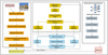 |
Fig. 1 Overall architecture and data flow of the intelligent control system. |
2.1 Dynamic state perception and data fusion module
2.1.1 Data collection and time series construction
The RTU (remote terminal unit) and the SCADA system onsite are synchronously capturing measurement points, such as pressure, flow, valve position, and gas quality, via Modbus TCP/IP. All terminal sampling uses a standard time base and is time-calibrated by the master control server. The original sample stream is then routed through a lightweight preprocessing pipeline, and presampling missing-value interpolation and presampling outlier removal are applied using median filtering before the sample stream enters the message queue (Kafka). Then, the continuous samples are reconstructed into time slices according to the configured window [27,28]. The time slice is divided into fixed steps Δt and forms the state sequence input, as shown in formula (1):
 (1)
(1)
Each data point x contains a location identifier and a multivariate measurement point vector. To eliminate short-term noise and sensor drift, an adaptive sliding mean filter is applied to the input. The filter window and weights are automatically adjusted based on the measurement point’s noise spectrum. All samples are uniformly normalized and written to a time-series database (InfluxDB), enabling low-latency subsequent feature processing and online training. This provides a highly consistent foundation for raw time series data.
2.1.2 Multi-source fusion and state extraction
Multi-source data have differences in spatial distribution and accuracy, so a weighted Kalman filter is used to achieve measurement fusion. The filter uses the SCADA overview measurement point as the benchmark observation and the field sensor as the local correction item. The weight is adaptively updated based on the observation covariance and the historical residual. State prediction and correction are performed by a linear transfer and observation model, respectively, thereby reducing the impact of abnormal measurement points on the overall estimation [29]. The feature dimension reduction is performed on the multidimensional vector after preliminary fusion. The principal direction is first extracted using principal component analysis (PCA), and then the importance of each variable is ranked using mutual information. The principal components with a cumulative contribution rate of at least 85% are retained as the candidate feature set. The retained features are normalized and spliced with time windows to generate the final input weight, as shown in formula (2):
 (2)
(2)
Each term represents pressure, flow, valve position, gas quality, and a risk indicator based on residuals and historical fluctuations. The risk indicator is quantified as a single scalar by summing the frequency and magnitude of anomalies within a sliding window, allowing subsequent policy modules to directly map safety constraints into the reward structure [30,31].
To achieve online state recognition, a cascade network of lightweight convolutional layers and gated recurrent units (CNN-GRU) is constructed to perform temporal classification on S̃ t. The convolutional layers extract local correlation patterns along the spatial dimension. In contrast, the GRU layers capture short- and medium-term dependencies. The output is a probability distribution of state categories and associated confidence scores. Network training uses a regularized cross-entropy loss combined with a mini-batch online update mechanism to adapt to data drift. A parallel residual threshold monitoring mechanism is also deployed: statistical boundaries are established based on the historical distribution of normal operation. When the real-time residual exceeds three times the standard deviation, an anomaly flag is triggered, and the event is written back to the training queue as a label for feedback training in the reinforcement learning module.
Figure 2 shows the results of two core experiments in dynamic state perception and data fusion. Figure 2a shows 24 h of pressure data, with time (h) on the horizontal axis and pressure (MPa) on the vertical axis. The results compare the original noise signal, the Kalman filter estimate, and the actual pressure change. The results show that the Kalman filter curve (blue line) effectively smooths high-frequency noise, and the overall trend closely matches the actual signal (red line), demonstrating that the algorithm can achieve accurate state estimation without losing dynamic characteristics. Figure 2b shows time (h) on the horizontal axis and flow rate (m3/h) on the vertical axis, demonstrating the effectiveness of time series anomaly detection in flow data containing abnormal disturbances. The anomalies marked by red dots correspond to system mutations or external interference. They are clearly distinguishable from normal fluctuations, validating the algorithm’s ability to identify anomalies under complex operating conditions. Figure 2 visualizes the comprehensive intelligent control performance of this study in dynamic state perception, noise suppression, and anomaly identification.
This module’s processing chain includes synchronous acquisition, preliminary cleaning, distributed caching, weighted fusion, principal component reduction, risk quantification, and time-series classification. All steps are pipelined and automated with low-latency transmission, ensuring that the environmental inputs received by subsequent policy learning meet the requirements of online training and real-time decision-making in terms of temporal consistency, noise suppression, and key feature representation. The module interface exposes normalized state vectors and event labels.
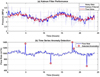 |
Fig. 2 Comparison of key dynamic state perception algorithm results. (a) Performance comparison of Kalman filtering in pressure signal denoising. (b) Traffic anomaly detection results based on time series analysis. |
2.2 Reinforcement learning intelligent decision engine
2.2.1 Dual-depth Q-network structure design
The reinforcement learning intelligent decision engine adopts a double deep Q-network (DDQN) architecture to address the policy oscillation and overfitting problems of traditional Q-learning in high-dimensional state spaces. The model is based on a value network composed of convolutional and fully connected layers that estimate the Q-value function for each state-action pair. The input vector is the standardized state sequence S̃ t output by the dynamic state perception module. The output layer dimension matches the number of executable actions, corresponding to operations such as valve opening adjustment, flow distribution, and pressure correction. The network uses the ReLU activation function and the Adam optimizer for parameter updates. The learning rate is set to α = 10‒4. To reduce the Q value estimation deviation, the target network and the main network separation mechanism are introduced to maintain the parameter set θ and θ′, respectively. The main network updates its parameters after each iteration, and the target network synchronizes its weights with a fixed step size N to ensure stable target estimation. The update formula is formula (3):
 (3)
(3)
where yt is the target Q value, γ is the discount factor, and rt is the immediate reward. The loss function uses the mean square error form, as shown in formula (4):
 (4)
(4)
Backpropagation minimizes the loss to update the main network parameters, approximating action values and enabling stable policy optimization. To avoid gradient explosion, weights are normalized during parameter updates to maintain numerical stability. An experience replay mechanism is used to break sample correlation and improve training efficiency. In each round of interaction, the system stores the samples (S̃ t, at, rt, S̃ t+1) into a circular buffer with a capacity of M. During training, small batches of samples are randomly sampled from the buffer for gradient updates. Sample priority is calculated using a dual-factor time-decay and error-margin approach, allowing the learning process to focus on high-reward samples early and converge to a stable policy later. Training continues until the average reward increment falls below a set threshold δr, indicating policy convergence. The key hyperparameters of the DDQN model on this platform are set as follows: experience replay pool capacity N = 10, batch size 64, discount factor γ = 0.99, target network update cycle τ = 100 steps, initial exploration rate ε = 1.0, and decay rate λ = 0.9995.
2.2.2 Strategy generation and online update mechanism
In emergency circumstances, action selection uses an ε-greedy strategy to balance exploration and exploitation. Initially, a high ε value is specified throughout training to encourage exploration of the action space, and thereafter, it gradually decreases according to an exponential decay function. The dynamic perception module inputs state data in real time to the system, estimates the action value, and takes the action with the maximum output. The result of an action execution is received by the environment, which generates a new state, forming feedback and enabling online closed-loop learning of the strategy. To address the non-stationary nature of the emergency, the strategy adjustment to the agent architecture via network parameters will perform soft replacements rather than hard replacements to avoid introducing strategy drift due to switching action policies. The weight update follows formula (5):
 (5)
(5)
where τ is the fine-tuning coefficient typically set to a 10‒3 level. This mechanism maintains progressive synchronization between the target network and the main network, enabling the policy to maintain a stable response under unexpected conditions. To improve the policy’s generalization, the system introduces state perturbations and random dropout mechanisms during training to add small amounts of noise to the input features. This ensures the model remains robust in unseen conditions.
Once on the platform, the network runs in online micro-batch mode that reads the latest state sequences from the database for short-term updates. Each training cycle is less than 10 s, enabling the network to produce the next action strategy in response to emergencies rapidly. The strategy output is sent to the control bus in JSON (JavaScript Object Notation) format for execution via commands that correct pressure or adjust valves at each node. Feedback is collected after execution, and the training cycle is reiterated. This process runs continuously in the system background to enable adaptive evolution of reinforcement learning strategies.
Figure 3 shows the performance development of the natural gas pipeline emergency control intelligent decision-making engine based on DDQN over training rounds. In Figure 3a, the horizontal axis represents training rounds, while the vertical axis shows the average Q-value. The Q-value stabilizes after about 600 training rounds, indicating that the agent’s action selection has stabilized. In Figure 3b, while the horizontal axis represents the number of training rounds, the left vertical axis indicates the cumulative reward. In contrast, the right vertical axis shows the exploration rate ε. As the number of training rounds increases, each cumulative return motivates the agent to use stable communication tactics to form a relatively optimal emergency dispatch strategy. At the same time, the exploration rate ε decreases, illustrating that the transition from random exploration at the beginning of training to the agent seeking to use stable communication tactics to form a relatively optimal emergency dispatch strategy occurs in stages. Figure 3c shows that the horizontal axis represents training iterations, and the vertical axis represents the loss on a logarithmic scale. The loss curve decreases exponentially and then stabilizes, indicating that the neural network’s parameters are gradually being optimized and that the learning process is stable. These results demonstrate that the constructed reinforcement learning decision-making engine can effectively achieve policy convergence in high-dimensional dynamic environments.
The entire decision-making engine is responsible for strategy generation and continuous optimization in the system architecture. Through the collaborative design of dual network separation, experience replay, and a soft update mechanism, it ensures faster strategy convergence and decision stability.
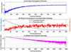 |
Fig. 3 Schematic diagram of the training process of the reinforcement learning intelligent decision engine. (a) Q-value convergence process. (b) Reward convergence and exploration strategy. (c) DDQN loss function downward trend. |
2.3 State-action adaptive mapping mechanism
2.3.1 State encoding and policy network construction
The state-action mapping process is based on the standardized state vector generated by the previous module S̃ t = [Pt, Qt, Vt, Ct, Rt]. To achieve continuous mapping between the state and action spaces, the system first performs dimension expansion and normalization encoding on the state variables at the input end, mapping variables of different dimensions to the interval [0, 1] to ensure consistent feature scales. Subsequently, a two-layer fully connected feedforward network is used to construct a state feature encoder with 256 and 128 hidden-layer nodes, respectively, and the activation function is LeakyReLU to maintain gradient continuity. The output layer is linearly transformed into a compressed feature representation vector ft, which serves as the input to the policy network, as shown in Formula (6):
 (6)
(6)
where W1 and W2 are the weight matrix, σ(.) is the activation function, and b1 and b2 are the bias terms. This feature-encoding structure provides a high-dimensional, nonlinear representation of state information, enabling subsequent action generation with continuous adjustment capabilities. The policy network is represented by a parameterized function π(at | Ŝt; θπ) and consists of a three-layer fully connected structure. The network outputs continuous action vectors at = [ΔPt, ΔQt, ΔVt] corresponding to the three dimensions of pressure regulation, flow distribution, and valve control. The network uses mean square error loss combined with policy gradient optimization, and the objective function is (7)
 (7)
(7)
where D represents the collection of samples from the experiences. The parameter optimization update uses gradient ascent, aiming to maximize the expected return of the behaviors executed by the policy based on the experiences collected to that point. Moreover, to limit oscillation, the final output is squashed within a Tanh function’s boundaries and multiplied by a control boundary matrix before execution, thus controlling the action within a safe range.
The policy network is trained using a parallel update procedure with the Q-network, where it collects experience after every action. It synchronizes state-feature encoding with action prediction. Then, the policy gradient direction is modified by the Q-network action. The following processes are completed asynchronously using multithreading, maximizing GPU usage to accelerate matrix operations and leveraging the GPU to improve policy mapping efficiency.
2.3.2 Action execution and adaptive feedback adjustment
To achieve adaptive adjustment of actions, the system introduces an error evaluation function in the feedback stage, such as formula (8):
 (8)
(8)
where Et represents the response deviation of the system state after executing the action. If the deviation exceeds the dynamic threshold δe, the policy fine-tuning process is triggered. The fine-tuning process updates the policy parameters θπ ′ through local retraining, performing backpropagation only for highly sensitive state variables to avoid global parameter fluctuations. For different emergency levels, the system sets an action-weight matrix Wa at the policy level, and the weights are dynamically adjusted based on the risk indicator Rt. As the risk level increases, the weight of pressure and flow adjustment actions increases, while the weight of valve position control decreases relatively, prioritizing system safety [32,33]. This weight update process is automatically executed after each policy evaluation, without requiring human intervention, to enable adaptive optimization of action allocation.
Figure 4a shows the flow response (Z-axis, m3/h) of a natural gas pipeline under different pressure (X-axis, MPa) and valve opening (Y-axis, %) conditions. The height of the curve indicates the system’s responsiveness to adjustments in action. The shape of the curve reveals the nonlinear coupling relationship between flow and pressure and valve changes: when the pressure is in the range of 3−5 MPa and the valve opening is in the range of 50%−70%, the flow peak reaches approximately 260 m3/h, indicating that the system has optimal control sensitivity and energy efficiency response within this range. Figure 4b shows the adaptive weighting changes of the system for the three objectives of safety, efficiency, and response over 24 h. The safety weight accounts for a larger proportion, and the weights of the three objectives vary periodically. The response weight remains relatively small, as seen in the dynamic balance of multiple objectives in the platform’s emergency control within 24 h.
The policy execution module and the reinforcement learning core engine operate out of order without synchronization. After each control cycle, execution feedback is written to the experience replay pool, where it informs the subsequent update of the learning network. This real-time closed-loop process provides millisecond-level feedback to the policy network, which is essential for continued learning and dynamic optimization. The long-term operation of the system maintains adaptive convergence, continuously reading and adjusting the mapping function parameters to ensure that the relationship between changes in the system’s state and changes in action responses remains optimal, enabling fast, accurate control actions across a variety of emergency conditions.
The valve control stability index measures the smoothness of the control strategy output. It is defined by the variation in valve-opening commands across multiple consecutive control cycles. Specifically, this index is calculated by taking the variance of the absolute-value sequence of valve command changes between adjacent cycles, normalizing it by the largest change in that sequence, and then subtracting the normalized variance from 1 to obtain the final value. The index ranges from 0 to 1; the closer the value is to 1, the smoother the valve command changes, the smaller the strategy oscillations, and the more reliable the control behavior.
 |
Fig. 4 State-action adaptive mapping mechanism diagram. (a) Action-state response surface. (b) Multi-objective adaptive weight adjustment. |
2.4 Multi-objective reward function design
2.4.1 Reward function structure construction and parameter normalization
To achieve dynamic control of the natural gas pipeline network under failure conditions, a multi-objective composite reward structure is introduced into the reinforcement learning decision-making process, considering safety constraints, scheduled timeliness, and energy efficiency as the primary optimization dimensions. After the normalization process, the state input and action output contribute to reward function calculations in normalized vectors. Each objective sub-function is modeled first independently and then weighted to create an overall reward term. Let the system reward function at time t be (9):
 (9)
(9)
where Rs(t), Rt(t), and Re(t) represent the safety, timeliness, and energy consumption target rewards, respectively, ws, wt, and we are weight coefficients, and Pt is the penalty term. The weight parameters are dynamically updated according to the system operation status and are implemented through a parameter smoothing mechanism based on soft updates, as shown in formula (10):
 (10)
(10)
where λ is the smoothing coefficient and  is the real-time evaluation weight. This mechanism suppresses weight fluctuations caused by unexpected conditions, ensuring the continuity and differentiability of the reward distribution and thereby improving the stability of policy gradient estimation. In the safety reward section, the system uses the deviation between the pipe pressure Pt and the valve opening Vt as the constraint. The target interval is set to Pmin and Pmax. If the actual pressure exceeds the range limits, we will apply a linear penalty equal to the excess. This design allows for the strategy to prioritize safety margins throughout the exploratory process. The timeliness reward ΔTt is calculated as the difference between the scheduling response time and the deadline. It is defined by an exponential decay function to mitigate the negative impact of response delay on the total reward. The energy consumption reward is calculated based on the energy consumption per unit flow rate ηt for the given time step and incurs a quadratic penalty for consumption exceeding the expected amount. All sub-functions are then calculated in parallel at the same time step and combined and normalized to produce a total reward signal.
The weights in the multi-objective reward function are adjusted using a dynamic adaptive mechanism. At the end of each control cycle, the system automatically reallocates the weights of the three sub-objectives—safety, timeliness, and energy consumption—based on the current risk level (quantified by the risk index defined in Sect. 2.1.2). The initial base weights are set as follows: safety 0.6, timeliness 0.2, and energy consumption 0.2. As the risk level increases, the safety weight increases, while the energy consumption weight decreases. The timeliness weight is slightly increased in low-to-medium risk phases to ensure response efficiency. Specifically, this adjustment is achieved by introducing three preset adjustment coefficients (safety gain coefficient 0.3, timeliness compensation coefficient 0.1, and energy consumption suppression coefficient 0.1): the higher the risk, the more prominent the importance of the safety objective, while energy consumption optimization is temporarily weakened, thus guiding the strategy to prioritize system safety.
2.4.2 Dynamic penalty mechanism and reward signal feedback adjustment
During the reinforcement learning training phase, if an action violates safety constraints or results in a sharp increase in energy consumption, a dynamic penalty mechanism is immediately triggered. The penalty value is determined based on the degree of deviation and the duration. By applying a time-decay factor γp, the system imposes a higher penalty on long-term accumulated deviations, thereby prioritizing the correction of persistent errors. The penalty term Pt is defined as in formula (11):
 (11)
(11)
where αp, αv, and αη are the penalty coefficients for each dimension, and γp controls the rate at which the penalty decays over time. This structure enables the system to achieve higher fault tolerance during the early exploration phase, while gradually strengthening safety constraints as the strategy stabilizes.
At each pass of the algorithm, the reward signal is stored in the experience replay pool, along with the state-action-next-state tuple, as context for gradient updates to the target network. Rewards are still averaged using a weighted methodology within each batch of training samples to retain some context for making policy updates to relative activities. Considering that rewards can often be sparse, small positive rewards are given during stable periods with no surprises to keep memory learning. To assist with the convergence of reward signals, adaptive reward scaling is employed to smooth them more efficiently. The average mean square error from the reward distribution will be used across the previous rounds. If the variance is too high, it automatically increases/decreases the scaling factor (within range) to provide a smoothed gradient estimate. The scaled reward is subsequently processed during the Q-network update phase, creating a continuous loop from the state-evaluation process to the reward-feedback process [34,35].
During the final training stages, sample data are used to recalibrate the reward function periodically. By measuring target completion rates across multiple emergency instances, the system adjusts the weight matrix to increase safety in high-risk situations and reduce effort and energy consumption during normal operation. This process is fully automated and requires no entry-level human intervention. In the end, the reward function finds an adaptive equilibrium between these objectives. It allows reinforcement learning decisions to converge and stabilize across multiple safety constraints, time responsiveness, and effort and energy budget management, thereby providing quantitative feedback for emergency response.
The multi-objective Pareto front is depicted in Figure 5, showing the distribution of feasible scheduling solutions across the three objectives: safety, efficiency, and energy consumption. The safety target value corresponds to the model’s response to valve regulation and pressure control concerning the safety constraints of the system; the efficiency target value denotes the level of scheduling efficiency the system achieved for specific safety constraints, whereas the efficiency level is conveyed through color mapping; and the energy consumption target value corresponds to energy consumption under various scheduling strategies. The points in Figure 5 represent all feasible solutions with respect to safety, efficiency, and energy consumption and illustrate the overall performance of a range of action combination strategies pertinent to a system in a specific state, with efficiency points shown in dark colors. The red points indicate the Pareto front, which reflects the strategy that yields the best balance across the three objectives, namely one that cannot improve the value of any single objective without sacrificing the value of another.
To quantify the optimization performance of the Pareto front, we introduce the hypervolume (HV) metric for evaluation. Using an ideal point (safety = 100%, efficiency = 100%, and energy consumption = 0%) as a reference, the calculated HV value for the Pareto solution set is 0.842 (normalized), significantly higher than 0.613 for rule-based systems and 0.721 for MPC, indicating that our proposed method achieves a better and more uniformly distributed solution set in the multi-objective space.
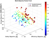 |
Fig. 5 Multi-objective Pareto front visualization. |
2.5 Platform architecture and visual control Interface
2.5.1 System overall architecture design and module integration
The platform’s overall design is structured into layers: a data acquisition layer, a smart decision-making layer, a control execution layer, and a visual interaction layer. The platform is primarily developed in Python, and the primary algorithmic framework uses TensorFlow. Deployment of the platform is based on a Linux cluster architecture that uses a container-based approach for each module, providing isolation and parallel scheduling while keeping each functional module independent and scalable. The data acquisition layer coordinates with SCADA and distributed sensor nodes using an asynchronous I/O communication mechanism, along with a multi-threaded acquisition engine, to provide high-speed acquisition of signals for pressure, flow, temperature, and valve position. The data access module transmits acquisition data in real time via Kafka streaming middleware. Once the data has been transmitted, preprocessing and exception detection use Spark Streaming to analyze it, then write the formatted data to PostgreSQL and InfluxDB time series databases.
The intelligent decision-making layer is part of the reinforcement learning core engine, which includes a state encoding module, a policy network, and a reward feedback unit. Modules communicate with each other using a RESTful API (application programming interface), achieving low-latency interaction with a small, lightweight data format (e.g., JSON). During inference, the system will leverage TensorFlow Serving to deploy the policy network model and use GPU parallelism to speed up policy time generation. The decision output is sent to the control execution layer through an intermediate buffer queue. The execution layer will call the underlying interface based on the policy’s action to complete valve adjustment and write the pressure regulation instruction. To prevent communication interruptions in the event of an emergency, the system includes breakpoint resumption and state snapshot recovery logic, allowing it to resume from the most recently saved safe state after restart.
The platform employs a task-scheduling approach based on a distributed task queue implemented with Celery. Centralized emergency tasks are scheduled by the scheduling manager, who handles the ordering of calls to multiple modules through a message queue. All logs related to computation and intermediate results are temporarily stored in Redis, enabling real-time tracking and logging of task execution, including exception backtracking. The data security layer supports end-to-end message encryption with AES (advanced encryption standard) to reduce command injection and data loss. The permission control module implements a user role hierarchy based on the RBAC (role-based access control) model to enforce hierarchical authorizations for administrative tasks, including, but not limited to, executing emergency actions, amending policies, accessing data, and setting platform access levels.
The system management terminal serves as a complementary system component to a console, providing log monitoring, task state monitoring, and a resource utilization dashboard to gauge the platform’s operating state, computing resource distribution, and operational status.
2.5.2 Visual control and interaction design
To enhance the platform’s training and review capabilities, this paper adds a log playback function for operator intervention strategies to the visual control interface. This function fully records the entire sequence of operations, timestamps, and snapshots of the system state at the time when the operator overwrites or adjusts the model’s output instructions during human-machine collaborative scheduling. The playback module supports frame-by-frame playback along the timeline, simultaneously displaying the model’s original suggestions, operator intervention actions, and the system’s subsequent response results. This provides schedulers with an intuitive comparative analysis tool for a deeper understanding of the consequences of different decision paths, effectively supporting post-event review, experience summarization, and new employee training.
The visual interface is based on a front-end and back-end architecture, using Vue and ECharts on the front-end and Flask on the back-end to provide a data interface. The visual interface consists of three area types: a status monitoring area, a policy control area, and a prompt alarm area. Each area contains three separate curves that visualize live trends in pressure, flow, and valve position (i.e., from open to closed), with data pushed via WebSocket and refreshed at near-millisecond intervals. The policy control area displays the model’s optimal action and expected reward outputs, as well as the operator’s ability to interject. The system records model outputs and human interventions for future retraining and policy adjustments.
When operating parameters exceed the operational limit threshold, the alarm module immediately displays the prompt and hyperlinks to the emergency response unit. The operator can engage the automatic control command highlighted in the interface, and the platform will send feedback and update the status curve after execution. The parameter adjustment area allows dynamic modifications to weights and control cycles, and all modifications are concurrently synchronized with the operation module after transactional verification. The system is structured to use the MQTT (message queuing telemetry transport) protocol to disseminate operational instructions to all nodes, ensuring consistent delivery of these instructions within each node. In the interactive display, the interface shows the exogenously generated optimal control action as a color gradient, indicating a gradual or sudden shift towards the desired action within the operations decision protocols.
Considering the needs of dispatchers without an AI background, this paper enhances the interpretability of strategy outputs in the strategy control area. When the model generates a critical control command (such as significantly adjusting valve opening or pressure setpoint), the system automatically generates a concise natural language explanation, such as: “Due to a detected sudden drop in upstream pressure (−1.2 MPa/s), to prevent downstream gas supply interruption, it is recommended to immediately open valve V-203 to 75%”. This explanation is calculated based on key features of the current state vector and real-time feedback from the reward function, helping operators quickly understand the direct reasons and expected goals behind the model’s decisions, thereby enhancing trust and efficiency in human-machine collaboration.
3 Results and discussion
The evaluation experimental data for this study come from historical operational records of a regional natural gas pipeline network and from emergency scenario data generated by the pipeline network simulation platform. The historical operational records include continuous sampling data on pressure, flow, valve opening, and compressor power, spanning different seasons, loads, and operating conditions across the pipeline network, with a total sampling time exceeding 1 year. Based on historical data, the simulation platform generates a variety of emergency event scenarios, including pipeline pressure drops, sudden valve closure, and flow anomalies. It generates time-series data consistent with the actual monitoring system through high-frequency sampling. All data are cleaned, missing values are imputed, and the data are normalized to form a complete state–action–feedback sample, which is used for online simulation and the verification of reinforcement learning strategies under different emergency conditions. Based on this dataset, this study systematically evaluates the performance of intelligent control across five aspects: response time, action stability, safety-constraint maintenance, energy consumption optimization, and strategy convergence and robustness. To enhance the engineering credibility of the research results, we collaborated with a provincial natural gas dispatch center in subsequent work to conduct a small-scale field deployment pilot. On a 12−km-long branch line containing three pressure regulating stations and two critical valves, this platform was embedded into its existing SCADA system for a six-week parallel operation test. During the test, the platform did not directly control the field equipment; instead, it generated scheduling suggestions in real time and compared them with manual scheduling instructions. Given the impact of climate and season on pipeline load and equipment response characteristics, we used historical operating records spanning all four seasons to divide the test set into quarters for retrospective verification. The results showed that the average response time in winter (high load period) was 1.08 s, slightly higher than in summer (0.89 s), mainly due to increased state fluctuations caused by frequent compressor start-ups and shutdowns; however, the safety retention rate remained stable in the range of 91%−93% in all seasons, indicating that the model has strong adaptability to seasonal operating conditions.
3.1 Evaluation of regulatory response timeliness
The experiment set up multiple emergency scenarios, including sudden valve closure, a drop in pipe pressure, and sudden changes in flow rate. After the platform activated the reinforcement learning strategy, it recorded the entire process latency from anomaly detection to the issuance of control commands. The system log automatically records the policy inference start time and execution confirmation time, and the average response time is calculated by comparing timestamps. To eliminate interference from communication factors, the platform separately sampled network transmission latency and excluded it from the calculation. The evaluation selected a fixed time window, statistically analyzed the latency distribution of 100 emergency cycles, and plotted a trend curve. Through multiple rounds of testing, the policy engine’s time stability is verified under different load conditions. The linear relationship between decision frequency and system load is also checked to ensure that the control system maintains a fast response characteristic under high-frequency, sudden conditions. The models evaluated in this paper are DDQN, DQN, Q-learning, PID (proportional–integral–derivative) control, rule-based system, MPC (model predictive control), expert system, and traditional optimization.
Figure 6 shows the response time of the industrial control system under different emergency scenarios and different algorithms. The horizontal axis of Figure 6a represents eight typical emergency scenarios, including sudden valve closure, pipe pressure drop, and sudden flow rate changes. In contrast, the vertical axis represents the system response time (s). It can be seen that the response times are highest in leakage events and compressor failures, approximately 1.44 and 1.45 s, respectively, while sudden valve closure and temperature anomaly scenarios have the fastest responses, with average response times of less than 1 second, reflecting the system’s sensitivity to different abnormal situations. The horizontal axis of Figure 6b represents eight control algorithms, while the vertical axis represents response time (s). The results show that the DDQN method in this paper has an average response time of approximately 0.96 s, significantly outperforming traditional Q-learning and rule-based systems, demonstrating the advantages of reinforcement learning in intelligent decision-making in improving control timeliness and emergency response speed.
To more clearly illustrate the system’s real-time performance, this paper provides a detailed breakdown of the end-to-end latency. The complete closed-loop latency from the occurrence of an abnormal event to the completion of the final control command execution consists of three main parts: perception latency (including data acquisition, transmission to the message queue, and preprocessing, averaging approximately 0.32 s), inference latency (i.e., the time required for the reinforcement learning policy engine to generate the optimal action, averaging approximately 0.41 s), and execution latency (covering command issuance, device physical response, and status feedback confirmation, averaging approximately 0.23 s). Optimizing these stages collectively ensures the system’s overall average fast-response capability of 0.96 s, with the perception and inference stages accounting for most of the total latency.
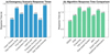 |
Fig. 6 Control response time evaluation. (a) Response time for different emergency scenarios. (b) Comparison of the response time of different algorithms. |
3.2 Action execution stability evaluation
The platform operates continuously, maintains a constant external disturbance intensity, and evaluates the smoothness of the output action by collecting valve-opening and pressure-control curves. During the evaluation process, the system records the action vector and actual execution feedback once per second. It calculates the differential sequence between the control instructions at the end of each cycle. If the amplitude of the change in the instructions of adjacent cycles is too large, it is determined that there is a strategy oscillation phenomenon in this stage. The test also monitors the execution unit’s feedback delay to ensure a linear mapping between the action output and the device response. Through multi-batch continuous operation verification, the stability trend of the control instructions across different training rounds is compared, and the degree of improvement in the network’s convergence on action stability is evaluated.
Table 1 presents the quantitative results of action execution stability across different training rounds. As the number of training rounds increases from 100 to 10,000, the valve control stability index increases from 0.65 ± 0.08 to 0.98 ± 0.01, and the pressure control stability index increases from 0.72 ± 0.06 to 0.99 ± 0.01, indicating that the reinforcement learning model gradually develops a more stable and accurate control strategy during training. At the same time, the command change rate decreases significantly from 12.5 ± 2.3% to 1.2 ± 0.3%, indicating that the output action tends to be smooth and the policy oscillation phenomenon is significantly reduced; the adjustment time is shortened from 15.3 ± 2.1 to 2.1 ± 0.4 s, reflecting a significant improvement in the system response speed and dynamic adjustment capability. Overall, as policy convergence improves, the control system shows a stable trend toward optimized action continuity and response timeliness.
Comparison of control action stability indicators under different training rounds.
3.3 Safety constraint retention rate evaluation
The safety constraint retention rate assessment assesses the proportion of pipeline network operating parameters that remain within the safety range under reinforcement learning control. The experiment sets dual threshold ranges for pressure and flow and monitors each node’s status in real time after executing the emergency strategy. The system records the pressure and flow values at each sampling point via the data acquisition module and counts the number of times they fall within the safety range. If any parameter exceeds the specified range, the system marks the violation and stores the corresponding status and action information. After the statistical cycle ends, the safety retention rate for each time period is calculated. During the test, verification is repeated at different emergency levels to assess the stability of strategy adjustments in high-risk scenarios. The results are used to judge the control effectiveness of the reinforcement learning model under safety constraints and the actual constraint effect of the penalty mechanism in the reward function.
Table 2 presents the system’s safety-constraint maintenance and related response indicators across six emergency levels, reflecting the control capabilities and enforcement effectiveness of the reinforcement learning scheduling strategy under varying risk intensities. As the emergency level increases from level 1 (normal) to level 6 (dangerous), the pressure safety maintenance rate decreases from 99.2% to 92.1%, the flow safety maintenance rate decreases from 98.8% to 91.2%, and the overall safety maintenance rate decreases from 99.0% to 91.7%. This indicates that despite increasing system difficulty under higher risk, the system still maintains a high level of safety overall. Concurrently, the number of violation events increases from just 2 to 52, the average recovery time increases from 3.2 min to 25.4 min, and the penalty mechanism trigger rate climbs from 0.5% to 15.2%. These key data indicate that as risk increases, control actions trigger constraint penalties more frequently, and the recovery cost significantly increases. Overall, the values in Table 2 demonstrate the proposed reinforcement learning platform’s efficient and stable control capabilities in both routine and mild emergencies, while also showing that, in high-risk scenarios, more policy adjustments and stronger penalty constraints are required to maintain system safety.
Statistical results of safety restraint retention rate under different emergency levels.
3.4 Energy consumption optimization effect evaluation
Energy consumption optimization is evaluated by comparing the rate of change in energy consumption per unit gas volume before and after emergency control. The platform sets a constant gas transmission demand in a simulated environment and compares the compression work and throttling loss of the traditional scheduling algorithm and the reinforcement learning strategy. During the test, the compressor load, motor power, and flow data are collected to calculate the energy consumption ratio for each time period. The control system maintains stable gas output and eliminates the impact of flow fluctuations on energy consumption. After each round of testing, the sampled data is imported into the analysis module to calculate the energy consumption reduction during the strategy operation phase. The evaluation results are verified by running data statistics for 48 consecutive hours to verify the improvement trend of the reinforcement learning strategy on energy efficiency under multi-node coordination, and to test the long-term consistency of the multi-objective reward function for the energy consumption suppression strategy.
Figure 7 shows the energy consumption optimization results for the pipeline network system using different algorithms. Figure 7a shows that under the same operating conditions, the DDQN algorithm achieves the lowest energy consumption per unit gas volume (approximately 83.4 kWh/1000 m3), which is 13.2% lower than the traditional rule-based system, demonstrating its high efficiency and energy-saving characteristics under the dynamic control strategy. Figure 7b further compares changes in energy consumption before and after optimization using distribution statistics. The baseline model is a rule-based system. It can be seen that after optimization, the energy consumption distribution shifts to the left overall, and the average energy consumption decreases from approximately 89.9 kWh/1000 m3 to 85.1 kWh/1000 m3, resulting in an energy saving rate of approximately 5.3%. This demonstrates that the proposed method offers advantages in reducing energy consumption and improving operating efficiency.
To make the energy consumption optimization results more valuable for industry reference, this paper compares the energy consumption indicators of this platform with current oil and gas industry standards. Based on the “Test and Calculation Method for Energy Consumption of Natural Gas Transmission Pipeline Systems”, this paper calculates the comprehensive energy consumption per unit gas transmission volume (kWh/1000 m3). Experimental results show that, under the same operating conditions, the average comprehensive energy consumption per unit gas transmission volume of this platform is 85.1 kWh/1000 m3, approximately 13.2% lower than the industry-standard benchmark for typical operating energy efficiency (approximately 98.0 kWh/1000 m3). This fully verifies that this method has significant energy-saving advantages while complying with industry standards.
 |
Fig. 7 Energy consumption optimization effect evaluation diagram. (a) Comparison of energy consumption per unit gas volume of different algorithms. (b) Comparison of baseline and optimized energy consumption distribution. |
3.5 Strategy convergence and robustness evaluation
Convergence and robustness evaluations are used to verify the model’s stability under various operating conditions and random perturbations. The platform loads multiple random perturbation scenarios, adds Gaussian Noise and burst data loss to sensor inputs, and observes the magnitude of changes in policy output and action execution. After each round of testing, the changes in the loss function and reward values are recorded to determine the convergence rate of policy updates. To assess generalization, the system reloads the model and performs inference under operating conditions outside the training set, statistically controlling for performance deviations. Output consistency is assessed through multiple perturbation experiments to evaluate the model’s ability to maintain stable policy outputs under complex input conditions. Robustness is ultimately evaluated based on convergence speed, output smoothness, and recovery time from anomalies.
Table 3 presents the model’s performance across several perturbation conditions, highlighting trends in convergence speed, average reward, anomaly recovery time, and generalization score. However, performance trends generally decrease as perturbation severity increases. In the baseline environment, the model converged rapidly under 1250 epochs, averaging a reward of 95.2 with a generalization score of 92.5. Moderate perturbations, such as 10% Gaussian noise or data loss, limit both the rate of convergence and the average reward, but the model still performs well. With more severe perturbations, such as a 500 ms delay in communication or a sensor failing, the reward and anomaly recovery rate decrease significantly, increasing the necessary recovery time to 28.3 and 32.8 s, respectively. Under the most complex perturbations, the model did not converge until 2150 epochs, with an average reward of 75.8 and a generalization score of 71.2, indicating that the model shows signs of coping with multiple disturbances.
The robust performance against mild and moderate disturbances is enabled by multidimensional collaborative optimization of the perception-decision-execution loop within the reinforcement learning control system. The DDQN is effective in convergence speed and action execution stability thanks to the target network, experience replay, and the reward function. The Tanh output constraints from the policy network, along with the dynamic bound matrix, provide continuous, smooth transitions among the control commands. Although higher degrees of disturbance, with an adherence to safety constraints of 91.7% and minimum worst-case violations in emergencies, extend considerably beyond rule-based systems practice, this performance is based on the safety weighting agent in the reward function and penalty mechanisms through observations as the behavior operates. The strategy also optimizes compressor operation, reducing energy consumption. The model displays limited ability to handle composite disturbances; therefore, this constitutes further opportunities for improvement, e.g., the inclusion of state reconstruction or uncertainty representations improves the model’s robustness behavior.
To address extreme communication disruption scenarios, we constructed a “disconnection-recovery” stress test model in a simulation environment: simulating a communication interruption between the main control server and 30% of remote RTU nodes lasting 5−30 min, during which a Level 6 emergency event (such as a main pipeline burst) was injected. The platform, through a local cache of the most recent state snapshot and in collaboration with edge nodes, initiated a degraded operation mode—utilizing only information from uninterrupted nodes to perform conservative control (such as closing the upstream main valve and maintaining minimum downstream gas supply). Tests showed that, on average, the system could resynchronize the entire network state and restore full control capabilities within 8.3 s after communication was restored, without any secondary safety incidents occurring.
In this paper, the “composite disturbance” scenario is defined as the simultaneous application of the following three types of disturbances: (1) 10% Gaussian noise is injected into the sensor data; (2) 10% of the sampling points are randomly discarded to simulate data loss; and (3) a fixed delay of 500 ms is introduced into the transmission of control commands. This combination simulates the situation in which communication, sensing, and execution links deteriorate simultaneously in real pipeline networks.
Strategy convergence and robustness performance indicators under different disturbance conditions.
4 Conclusion
This study explores proactive management of natural gas pipeline systems during emergencies and develops an intelligent scheduling and control interface based on reinforcement learning. A multi-source data fusion and state-awareness module was developed to enable real-time acquisition and dynamic sensing of pressure, flow, valve position, and gas quality data. An optimal control strategy was developed using a dual-deep Q-network and a state-action adaptive mapping method. A multi-objective reward function was constructed to achieve safe control, timely scheduling, and efficient operation. Furthermore, a visual control interface for human-machine collaborative scheduling was developed. All quantifiable objectives of this study were achieved: average platform response time of 0.96 s, valve control stability of 0.98, settling time of 2.1 s, safety retention rate of 91.7% under Level 6 emergency conditions, energy consumption reduction of 13.2%, and benefit of 75.8% under complex disturbances. At the research step level, the dynamic perception module achieves low-latency fusion of multi-source data through Kalman filtering and PCA, providing high-quality state input for reinforcement learning; the DDQN decision engine converges within 600 rounds with a single-step inference time of 0.41 s, meeting the real-time requirements for emergency response; the adaptive mapping mechanism achieves valve/pressure control stability of 0.98/0.99; and the Pareto hypervolume of the multi-objective reward function is 0.842, significantly better than MPC (0.721) and rule-based systems (0.613). This research provides a deployable intelligent solution for emergency dispatching of natural gas pipeline networks, significantly improving system resilience and energy security. Future research will extend to multi-energy coupled systems of electricity, gas, and hydrogen, introducing transfer learning to enhance generalization capabilities and combining digital twins to achieve predictive closed-loop control.
Acknowledgments
Not applicable.
Funding
No funding was received for conducting this study.
Conflicts of interest
The authors declare no conflict of interest.
Data availability statement
This article has no associated data generated and/or analyzed/data associated with this article cannot be disclosed due to legal/ethical/other reason.
Author contribution statement
Huichao Guo, Runhua Huang, and Yanzhi Huang wrote the manuscript. All authors contributed to editorial changes in the manuscript. All authors read and approved the final manuscript.
References
- L. Fan, H. Su, W. Wang, Zio. E, L. Zhang, Z. Yang, S. Peng, W. Yu, L. Zuo, J. Zhang, A systematic method for the optimization of gas supply reliability in natural gas pipeline network based on Bayesian networks and deep reinforcement learning, Reliab. Eng. Syst. Saf. 225, 108613 (2016) [Google Scholar]
- W Shouxi, D Chuanzhong, C Chuansheng, W. Li, J. Li, X. Gao, Online simulation of natural gas pipeline networks: theories and practices, Oil Gas Storage Transport. 41, 241–255 (2022) [Google Scholar]
- C. Zhou, Z. Yang, G. Chen, G. Zhang, Y. Yang, Study on leakage and explosion consequence for hydrogen blended natural gas in urban distribution networks, Int. J. Hydrogen Energy 47, 27096–27115 (2022) [CrossRef] [Google Scholar]
- Z. Wang, Y. Kong, W. Li, Review on the development of China’s natural gas industry in the background of “carbon neutrality. Nat. Gas Ind. B 9, 132–140 (2022) [Google Scholar]
- X. Cao, T. Cao, Z. Xu, B. Zeng, F. Gao, X. Guan, Resilience constrained scheduling of mobile emergency resources in electricity-hydrogen distribution network, IEEE Trans. Sustain. Energy 14, 1269–1284 (2022) [Google Scholar]
- M. Cao, C. Shao, B. Hu, K. Xie, W. Li, L. Peng, W. Zhang, Reliability assessment of integrated energy systems considering emergency dispatch based on dynamic optimal energy flow, IEEE Trans. Sustain. Energy 13, 290–301 (2022) [CrossRef] [Google Scholar]
- Y. Mahmood, T. Afrin, Y. Huang, N. Yodo, Sustainable development for oil and gas infrastructure from risk, reliability, and resilience perspectives, Sustainability 15, 4953 (2023) [Google Scholar]
- C.A. Arinze, V.O. Izionworu, D. Isong, C.D. Daudu, A. Adefemi, Integrating artificial intelligence into engineering processes for improved efficiency and safety in oil and gas operations, Open Access Res. J. Eng. Technol. 6, 39–51 (2024) [Google Scholar]
- D. Wang, S. Shi, J. Lu, Z. Hu, J. Chen, Research on gas pipeline leakage model identification driven by digital twin, Syst. Sci. Control Eng. 11, 2180687 (2023) [Google Scholar]
- I.I. Bosikov, N.V. Martyushev, R.V. Klyuev, I.A. Savchenko, V.V. Kukartsev, V.A. Kukartsev, Y.A. Tynchenko, Modeling and complex analysis of the topology parameters of ventilation networks when ensuring fire safety while developing coal and gas deposits, Fire 6, 95 (2023) [CrossRef] [Google Scholar]
- L. Li, Development of natural gas industry in China: review and prospect, Nat. Gas Ind. B 9, 187–196 (2022) [Google Scholar]
- L. Cao, AI and data science for smart emergency, crisis and disaster resilience, Int. J. Data Sci. Anal. 15, 231–246 (2023) [Google Scholar]
- N.A. Eremin, D.A. Selenginsky, On the possibilities of applying artificial intelligence methods in solving oil and gas problems, Izv. Tulsk. Gos. Univ. Nauki o Zemle 1, 201–210 (2023) [Google Scholar]
- X. Xie, Y. Tian, G. Wei, Deduction of sudden rainstorm scenarios: integrating decision makers’ emotions, dynamic Bayesian network and DS evidence theory, Nat. Hazards, 116, 2935–2955 (2023) [Google Scholar]
- H. Meng, X. Meng, D. Li, S. Zhao, E. Zio, X. Liu, J. Xing, A STAMP-Game model for accident analysis in oil and gas industry, Pet. Sci. 21, 2154–2167 (2024) [Google Scholar]
- J.H. Corbin, U.E. Oyene, E. Manoncourt, H. Onya, M. Kwamboka, M. Amuyunzu-Nyamongo, K. Sørensen, O. Mweemba, M.M. Barry, D. Munodawafa, Y.V. Bayugo, Q. Huda, T. Moran, S.A. Omoleke, D. Spencer-Walters, S.V.d. Brouckeet, A health promotion approach to emergency management: effective community engagement strategies from five cases, Health Promot. Int. 36, i24–i38 (2021) [Google Scholar]
- Z. Wang, Y. Zhang, N. Li, J. Zhang, Spatiotemporal patterns and drivers of carbon emissions from on-site wastewater treatment: Evidence from a city-wide long-term network. Environ. Res. 296, 123948 (2026) [Google Scholar]
- D. Zhang, Development prospect of natural gas industry in the Sichuan Basin in the next decade, Nat. Gas Ind. B 9, 119–131 (2022) [Google Scholar]
- S. Peng, R. Chen, B. Yu, M. Xiang, X. Lin, E. Liu, Daily natural gas load forecasting based on the combination of long short term memory, local mean decomposition, and wavelet threshold denoising algorithm, J. Nat. Gas Sci. Eng. 95, 104175 (2021) [CrossRef] [Google Scholar]
- H. Zhang, Z. Tian, Failure analysis of corroded high-strength pipeline subject to hydrogen damage based on FEM and GA-BP neural network, Int. J. Hydrogen Energy 47, 4741–4758 (2022) [Google Scholar]
- Q. LEI, D. Weng, G.B. Guan, J. Shi, B. Cai, C. He, Q. Sun, R. Huang, Shale oil and gas exploitation in China: Technical comparison with US and development suggestions, Pet. Explor. Dev. 50, 944–954 (2023) [Google Scholar]
- O.F. Al Kurdi, A critical comparative review of emergency and disaster management in the Arab world, J. Bus. Socioecon. Dev. 1, 24–46 (2021) [Google Scholar]
- E.B. Priyanka, S. Thangavel, X.Z. Gao, Review analysis on cloud computing based smart grid technology in the oil pipeline sensor network system, Pet. Res. 6, 77–90 (2021) [Google Scholar]
- A. Kopbayev, F. Khan, M. Yang, S.Z. Halim, Gas leakage detection using spatial and temporal neural network model, Process Saf. Environ. Prot. 160, 968–975 (2022) [Google Scholar]
- J. Zhu, J. Pan, Y. Zhang, Y. Li, H. Li, H. Feng, D. Chen, Y., Kou, R. Yang, Leakage and diffusion behavior of a buried pipeline of hydrogen-blended natural gas, Int. J. Hydrogen Energy 48(30), 11592–11610 (2023) [CrossRef] [Google Scholar]
- W. Huang, X. Zhang, K. Li, N. Zhang, G. Strbac, C. Kang, Resilience oriented planning of urban multi-energy systems with generalized energy storage sources, IEEE Trans. Power Syst. 37, 2906–2918 (2021) [Google Scholar]
- Wang, Z., Wang, Y., Xiao, et al., Multi-time scale optimisation strategy for effective control of small-capacity controllable devices in integrated energy systems. Cyber-Phys. Syst. 11, 67–92 (2025) [Google Scholar]
- M. Farghali, A.I. Osman, I.M.A. Mohamed, Z. Chen, L. Chen, I. Ihara, P.S. Yap, D.W. Rooney, Strategies to save energy in the context of the energy crisis: a review, Environ. Chem. Lett. 21, 2003–2039 (2023) [Google Scholar]
- Q. Lei, Y. Xu, Z. Yang, B. Cai, X. Wang, L. Zhou, H. Liu, M. Xu, L. Wang, S. Li, Progress and development directions of stimulation techniques for ultra-deep oil and gas reservoirs, Pet. Explor. Dev. 48, 221–231 (2021) [Google Scholar]
- C. Howard, A.J. MacNeill, F. Hughes, L. Alqodmani, K. Charlesworth, R.d. Almeida, R. Harris, B. Jochum, E. Maibach, L. Maki, F. McGain, J. Miller, M. Nirmala, D. Pencheon, S. Robertson, J.D. Sherman, J. Vipond, H. Yin, H. Montgomery, Learning to treat the climate emergency together: social tipping interventions by the health community, Lancet Planet. Health 7, e251–e264 (2023) [Google Scholar]
- E.C. Onukwulu, M.O. Agho, N.L. Eyo-Udo, Sustainable supply chain practices to reduce carbon footprint in oil and gas, Glob. J. Res. Multidiscip. Stud. 1, 24–43 (2023) [Google Scholar]
- N. Norouzi, Post-COVID-19 and globalization of oil and natural gas trade: challenges, opportunities, lessons, regulations, and strategies, Int. J. Energy Res. 45, 14338–14356 (2021) [Google Scholar]
- T. Van Hoang, Impact of integrated artificial intelligence and internet of things technologies on smart city transformation, J. Tech. Educ. Sci. 19, 64–73 (2024) [Google Scholar]
- R. Li, W. Gong, L. Wang, C. Lu, Z. Pan, X. Zhuang, Double DQN-based coevolution for green distributed heterogeneous hybrid flowshop scheduling with multiple priorities of jobs, IEEE Trans. Autom. Sci. Eng. 21, 6550–6562 (2023) [Google Scholar]
- C. Zhou, Y. Huang, K. Cui, X. Lu, R-DDQN: optimizing algorithmic trading strategies using a reward network in a double DQN, Mathematics 12, 1621 (2024) [Google Scholar]
Cite this article as: H. Guo, R. Huang, Y. Huang, Development of a dynamic control and dispatching platform for natural gas pipeline emergency situations based on reinforcement learning, Mechanics & Industry 27, 20 (2026), https://doi.org/10.1051/meca/2026015
All Tables
Comparison of control action stability indicators under different training rounds.
Statistical results of safety restraint retention rate under different emergency levels.
Strategy convergence and robustness performance indicators under different disturbance conditions.
All Figures
|
Fig. 1 Overall architecture and data flow of the intelligent control system. |
| In the text | |
|
Fig. 2 Comparison of key dynamic state perception algorithm results. (a) Performance comparison of Kalman filtering in pressure signal denoising. (b) Traffic anomaly detection results based on time series analysis. |
| In the text | |
|
Fig. 3 Schematic diagram of the training process of the reinforcement learning intelligent decision engine. (a) Q-value convergence process. (b) Reward convergence and exploration strategy. (c) DDQN loss function downward trend. |
| In the text | |
|
Fig. 4 State-action adaptive mapping mechanism diagram. (a) Action-state response surface. (b) Multi-objective adaptive weight adjustment. |
| In the text | |
|
Fig. 5 Multi-objective Pareto front visualization. |
| In the text | |
|
Fig. 6 Control response time evaluation. (a) Response time for different emergency scenarios. (b) Comparison of the response time of different algorithms. |
| In the text | |
|
Fig. 7 Energy consumption optimization effect evaluation diagram. (a) Comparison of energy consumption per unit gas volume of different algorithms. (b) Comparison of baseline and optimized energy consumption distribution. |
| In the text | |
Current usage metrics show cumulative count of Article Views (full-text article views including HTML views, PDF and ePub downloads, according to the available data) and Abstracts Views on Vision4Press platform.
Data correspond to usage on the plateform after 2015. The current usage metrics is available 48-96 hours after online publication and is updated daily on week days.
Initial download of the metrics may take a while.