| Issue |
Mechanics & Industry
Volume 21, Number 6, 2020
|
|
|---|---|---|
| Article Number | 601 | |
| Number of page(s) | 18 | |
| DOI | https://doi.org/10.1051/meca/2020073 | |
| Published online | 22 September 2020 | |
Regular Article
Numerical analysis of thermal stresses and strains of annular finned tube bundle in turbulent flow regime
1
Faculty of Mathematics, University of Sistan and Baluchestan, Zahedan, Iran
2
Faculty of Engineering (Shahid Nikbakht Engineering Facutly), Department of Mechanical Engineering, University of Sistan and Baluchestan, Zahedan, Iran
* e-mail: This email address is being protected from spambots. You need JavaScript enabled to view it.
Received:
19
December
2019
Accepted:
27
August
2020
Abstract
In this paper, the effect of turbulent flow on the thermal stresses and strains created in an annular finned-tube bundle is studied. The finite volume method and the transition SST model, along with the SIMPLE algorithm, are used to solve the flow equations, and the finite element method is used to solve the thermal stress equations in solid. The results obtained from the effective stress and strain in the annular fins bundle show that despite the temperature difference of less than 1 degree between the base and the edge of the fin, the amount of thermal stresses cannot be ignored and the asymmetric distribution of temperature in the fins leads to the shear stresses which play a key role in determining the maximum position of the effective stresses in some rows. The results show that the amount of effective stress and strain in the third and fourth rows are significantly smaller than the first and second rows. The results also show that the highest amount of the effective stress occurs in the first row and the fin base at zero-degree angle, the value of which is 0.6 MPa. The predominance of the tangential stresses at the fin base in this row is the cause of this issue. However, in the second fins onwards, although the tangential stresses are still higher, the greater asymmetry of the temperature around the fins in these rows leads to comparability of the shear stresses with tangential stresses and creates the maximum effective stress at angles other than zero degree. Therefore, according to the results of this paper, the analysis of the flow around the annular fins is necessary to calculate thermal stress and strains and it determines the vulnerable points in each tube row. It is natural that with increasing temperature difference between the base and the edge of the fin and with increasing fin hight, the importance of these studies increases.
Key words: Finite element method / finite volume method / annular fin / thermal stress / thermal strain / turbulent flow / flow around finned tubes bank
© AFM, EDP Sciences 2020
1 Introduction
Today, the use of tubes bundle is one of the common methods for heat transfer in industry. The extensive use of the tubes bundle in industry has led researchers to conduct numerous research to increase the efficiency of the tubes bundle. One of the methods that is used today to improve the performance of the tubes bundle in the field of the heat transfer is to place the fins on the bundle of tubes. But on the other hand, the temperature gradient created in the fins increases the stress. This has led researchers to conduct several studies on the thermal stresses in the tubes and fins. In the following, we will review some of the research done in the field of examining the thermal stresses in the annular fins and studying the flow in the annular finned-tube bundle.
First, let's refer to some of the studies that have been done to investigate the distribution of temperature and the thermal stress in the annular fin with no flow. Using two methods of the inverse Laplace transform and the Simpson rule, Shang Sheng [1], studied the thermal stresses in a homogeneous and isotropic annular fin under the assumption of one-dimensional and transient heat transfer. Also Yu and Chen [2] investigated the stress distribution and the heat transfer in isotropic annular fin in one-dimensional mode with the convective, radiative, and convective-radiative boundary conditions in both steady and transient modes using hybrid method. They compared the temperature distribution and thermal stress obtained with different boundary conditions. Chiu and Chen [3] also used the analytical method to investigate the distribution of the temperature and thermal stresses in an isotropic annular fin. Their results showed that small temperature variations also cause significant differences in the thermal stresses. Using the homotopy analysis method, Aksoy [4] also examined the temperature distribution in an annular fin and compared the temperature distribution results with the finite difference numerical method. Roy and Ghosal [5] also used the method of homotopy perturbation to investigate the temperature distribution in the annular fin and the effect of temperature-dependent variations in the thermal conductivity coefficient on the efficiency of the fin and its temperature distribution. Peng and Chen [6] also investigated the distribution of temperature in an annular fin using the hybrid differential transform and the finite difference methods. Among the other research we can refer to the study by Aziz [7]. He solved the two-dimensional conduction in a rectangular fin and examined the effects of the presence of a thermal source, the non-uniform temperature of the fin base, and the variations in the thermal conductivity coefficient. Lau and Tan [8] also studied errors in one-dimensional analysis of heat transfer in straight annular fins. They presented a two-dimensional analytical solution for a fin under constant base temperature and the uniform thermal conductivity coefficient around the fin. Among other research that studied the temperature distribution and thermal stress in the annular fins, it can be mentioned to references [9–12].
We now turn to a number of studies that have examined the flow and heat transfer at annular finned-tube bundle. Jang et al. [13] experimentally and numerically studied the thermal performance of annular finned-tube bundle in 4 rows in dry and humid conditions at input velocity of 1–6 m/s. Their studies show that increasing the fluid velocity and one-dimensional fin assumption cause the error in approximation of the fin efficiency increase. Neal et al. [14] examined the heat transfer and flow behaviors of a nine-row annular finned-tube bundle. Mon and Gross [15] also numerically examined the effect of fin pitch on heat transfer, pressure drop, and flow field in four-rows annular finned-tube bundle with turbulent flow. Their results showed that the expansion of the boundary layer on the fin and the tube surfaces is essentially dependent on the ratio of the fin pitch to the fin height and also show that in linear arrangement when this ratio increases, the heat transfer coefficient increases and the pressure drop decreases. Bilirgen et al. [16] also repeated the research by Mon and Gross for a row annular finned-tube bundle with turbulent flow and examine more precisely the effect of Reynolds number and the effect the fin pitch, fin height, fin thickness, and fin material on pressure drop and heat transfer. Their results showed that the effect of the fin thickness on heat transfer and pressure drop is much less than the fin height and fin pitch. Jang and Yang [17] also studied the pressure drop and heat transfer at different input velocities (from 2 to 7 m/s) in the annular and elliptical finned-tube bundles by the numerical and experimental methods. They showed that the heat transfer coefficient of the annular finned-tube is 20 to 50% higher than that of the elliptical finned-tube with similar tubes. However, the pressure drop in the annular tubes is much higher than in the elliptical tubes. Hu and Jacobi [18] also conducted numerical-experimental study on heat transfer on a four-row annular finned-tube bundle. Their results indicated that at Reynolds number between 3,300 and 12,000, even if the angle of attack was very small, there would be a significant change in convective mass transfer and mass transfer behavior. Kuntysh and Stenin [19] repeated the study by Hu and Jacobi under turbulence flow assumption. Mon [20] also investigated the effect of geometry parameters such as the fin thickness, fin height, tube diameter, fin spacing, the fluid velocity and the fin arrangement of the annular finned-tube bundle on the heat transfer coefficient. The results showed that in linear arrangement, by increasing the ratio of the fin spacing to fin height, the heat transfer coefficient increases and the pressure drop decreases, while in the staggered arrangement, the heat transfer coefficient first increases and then decreases. Shokouhmand et al. [21] also investigated the optimization of the annular finned-tube bundle using constructal design method. Their goal was to find the optimal geometry to increase heat transfer. They showed that the optimal geometry is influenced by the flow condition. Nemati and Moghimi [22] also studied the numerical flow at the finned-tubes bundle in the heat exchangers with different models of flow turbulence. Their results showed that the Transition SST model is well compatible with the experimental results. Also, Nemati and Samivand [23] used the Transition SST model to study the flow and heat transfer in annular and elliptical finned-tube. Pis'Mennyi [24] also investigated the thermal and hydraulic performance of bent finned-tubes bundle in different directions. The results showed that using proposed levels significantly reduced the amount of metal and the size of the heat transfer equipment. As known, the fin back region in streamwise direction does not contribute much to the heat transfer. For this reason, Kuntish and Kuzentsov [25] removed the back part of the fins. Their results showed that this increased the heat transfer coefficient. However, decrease in heat exchange level leads to decrease in heat transfer rate, especially for high Reynolds numbers.
Finally, an overview of other research on the solving fluid flow problems and thermal stresses is given simultaneously. Wang et al. [26] used the liquid-solid-thermal coupling to investigate heat transfer and heat stress distribution along a tube of coil heat exchanger. Their results showed that as the velocity of the input flow increased, the heat transfer increased and the temperature difference decreased. Their results also showed that reducing the temperature difference lead to reduce the amount of thermal stress and increase the effect of the initial stress. Zhang et al. [27] used numerical and experimental methods to investigate the thermal performance and mechanical properties in plate-fins heat exchangers. They obtained the flow contours, pressure drop and temperature difference in their models. Demirdzic et al. [28] proposed a numerical method that can be used to analyze stress in a solid object and to predict fluid flow, both independently and coupled with a solid. They solved an example of a solid-coupled fluid flow in order to demonstrate the full capabilities of their method. Alzaharnah et al. [29] investigated the thermal stresses caused by the temperature distribution in the tube. They studied their problem under a fully developed flow assumption and a laminar flow field with constant properties inside the tube, and examined the problem as the symmetric axial problem with a uniform heat flux of 1300 W/m2 on the outer wall with an inlet fluid temperature of 293 K. They investigated the effect of diameter, thickness and length of the tube on the thermal stresses created in three different compositions and 27 different samples. Their results showed that the thickness of the tube wall and the tube diameter are important parameters that affect the thermal stresses of the tube. Hosseini et al. [30] investigated the thermal stresses and strains in a fin by passing an external flow over it. They used periodic boundary conditions to model a fin. They analyzed their problem in two regimes: the laminar and turbulence flow in transient way. Their results showed that during turbulent flow, the thermal stresses were much higher than the laminar flow, and the effect of flow on thermal stresses cannot be ignored.
According to the review of the literature it can be observed that some researchers limited their studies to the computation of the temperature [1–8] and the distribution of the thermal stresses and strains [1–3] on an annular fin in which the temperature distribution is one-dimensional in the fin. On the other hand, a number of researchers [13–25] have only studied the heat transfer and flow behaviors in the annular finned-tube bundle. Finally, some papers examined the flow inside the tubes [26–29] or the flow outside on a fin [30]. Although they related to both fluid flow and thermal stresses simultaneously, the thermal stresses and strains in the fin bundle have not been investigated. Therefore, the innovation of the present paper can be expressed as follows:
-
Investigating the effect of turbulence flow on each of annular fin in four row finned-tube bundle.
-
Investigating the effect of different shapes of fins on the thermal effeciency of the bank of finned tubes and the thermal stresses created in the annular fins.
-
Finally, finding the best fin's shape in reducing the thermal stresses created in fin with the highest thermal stress.
2 Problem description and governing equations
2.1 Problem description
In the present study, an annular fin bundle with boundary and geometric conditions, distance from the flow inlet (a = 23.8 mm), distance from flow outlet (b = 105.4 mm), solution domain height (h = 2.5 mm), solution domain width (c = 40.8 mm), two fin spacing (d = 6.8 mm) shown in Figure 1A–C, is studied. Other geometrical characteristics and the material properties of the fin are shown in Table 1. The temperature of the tube wall is also constant and equal to the temperature of the fin base. The airflow is turbulent, incompressible, constant and three-dimensional. Also, the fin is assumed homogenous and isotropic. Solution of the fluid area in the present study is done with the boundary conditions shown in Figure 1A–C using the FVM method and the Transition SST model [22] and the solid area is also done using the FEM method. Also, since the thickness of the fin is small, the governing equations in the solid area are solved with the assumption of plane stress. The geometric and the boundary conditions of the fluid domain are in accordance with the reference [22]. ANSYS Fluent and ANSYS Mechanical software [31] with Fluid-structural method iteration was used for numerical solution.
 |
Fig. 1 Annular finned tube bundle (A) X1–X3 plane, (B) X1-X2 plane, (C) a distinct fin. |
Thermal and geometric and material properties of the aluminum fins.
2.2 Governing equations and boundary conditions
2.2.1 Fluid domain
The governing equations of heat transfer in turbulent, steady, and incompressible fluid flow are as follows [22]:
A − Continuity equation: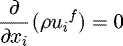 (1)
(1)
B − Momentum equation: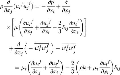 (2)
(2)
In equation (2), μ is the dynamic viscosity, μt is the turbulent viscosity, and k is the turbulent kinetic energy.
C − Energy equation: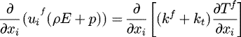 (3)
(3)
In equation (3), E is the total energy.
D − Boundary conditions
1. Inlet and outlet boundary conditions:
At the inlet, the fluid flow is uniform and in the direction of x1, with a temperature of 308.15 K, 1% turbulence intensity, and 2% turbulent viscosity ratio. At the outlet, the relative pressure is considered to be zero.
2. At the surfaces shown in Figure 1, the symmetry boundary condition is defined as follows.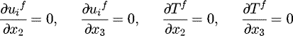 (4)
(4)
3. The no-slip condition defined for the tube and the fin is: (5)
(5)
In equations (4) and (5), u i f is the component i of the fluid velocity.
2.2.2 Solid domain (fin)
The governing equations of the solid domain (fin) include the energy equations, equilibrium equations, structural equations, and strain-displacement equations. The boundary conditions used to solve the energy equation are the thermal boundary condition of the constant temperature at the fin base and the boundary condition of the coupling between the fin and the fluid. Also, the condition of zero radial stress in the inner and outer radius and zero axial stress in the perpendicular to the fin to solve equilibrium equations and structural equations of the material is in the z direction. In addition, the important governing assumptions on the problem include the independence the heat equations from stress equations. This means that the energy equation is first solved using thermal boundary conditions and then equilibrium, strain-displacement and structural equations are solved using the calculated temperatures of the energy equation, with the mentioned boundary conditions of stress. Now, according to the stated explanations, the governing equations of the solid domain (fin) are as follows.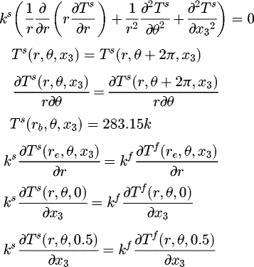 (6)
(6)
In equation (6), Ts
is the temperature, ρ
s
is the density, ks
is the thermal conductivity, and  is the special heat capacity of the fin. Also, for modeling of solid part, constitutive and equuilibrium equations [30] are used.
3 Grid and validation
3.1 Grid
Grid independence is checked for inlet velocity 2m/s and Reynolds number 9058. The grid independence section, griding, starts from the basic mesh 1630748 including the number of 686000 solid grid and 944748 the fluid grid. It should also be noted that in the present work, Fluid-structural interation method is used to the fluid and solid boundary meshes are compatible. The number of nodes is increased in a several steps until there is no change in the results after that number to ensure the selected grid. The type of the griding is shown in Figures 2 and 3. Structured grid is used in the space around the fins and the depth of the computational range. In each grid during the solution, the grid is modified to reduce the amount of y + to less than 5. Table 2 shows the results of the grid independence. As shown in Table 2, grid 4 can be selected as the appropriate mesh. The value of y + in grid 4 is 1.15.
 |
Fig. 2 Grid type defined for the fins. |
 |
Fig. 3 Grid type defined for the fluid domain and fin-fluid interface. |
Mesh Independence.
3.2 Validation
3.2.1 Fluid domain
To ensure the accuracy of the fluid domain solution results, the obtained numerical results and the experimental results are examined in three different Reynolds numbers. The following experimental relationships are used to predict the Nusselt number in an annular finned-tube bundle. The acceptable error rate for these relationships is also mentioned. As shown in Table 3, the highest error is with reference [33], which does not exceed 14.96%. In this way, the error obtained is in the acceptable range of 25%. The formula |a
i
− b
i
|/a
i
× 100 is also was used to calculate the relative error.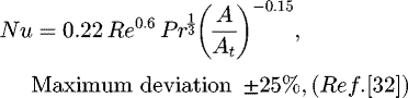 (7)
(7)
 (8)
(8)
Validation results for the fluid domain.
3.2.2 Solid domain
Figure 4 shows a schematic figure of the fin studied by Mallick and Das [9]. They considered the dimensionless boundary conditions shown in Figure 4 for their problem. The aim was to calculate the dimensionless temperature distribution and to calculate the thermal stresses in the annular fin. They used the SIMPLEX SEARCH METHOD to solve their given problem. Then, they compared the obtained results from their model with the results of Chiu and Chen [3] study in order to validate their model. Since the model used in Mallick and Das [9] study has been validated for all temperature conditions (they solved problem with boundary conditions in dimensionless mode), so if the present study is validated with Mallick and Das [9] work, the model used in the present work can also be applied for different temperature conditions and different temperature range of fins. Figures 5–7 show the comparison of the temperature distribution and thermal stresses of the present study with the results of both Mallick and Das [9] and Chiu and Chen [3] research, which indicates the accuracy of the numerical method used in the present study. In Figure 8, the results of the present numerical method are compared with the results of reference [9] study with different temperature conditions of the fin tip. As can be seen, the error between the two methods in the temperature distribution is less than 1.5%. According to the studies, the numerical method used for solving the thermal stresses in solid can be used for the given temperature conditions in the fins bundle, which is discussion subject in this paper.
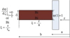 |
Fig. 4 Geometry of an annular fin having inner radius a and tip radius b. |
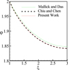 |
Fig. 5 Comparison of temperature values. |
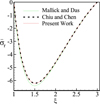 |
Fig. 6 Comparison of radial stress. |
 |
Fig. 7 Comparison of tangential stress. |
 |
Fig. 8 Comparison of temperature values. |
4 Results and discussion
In this section, the contours of temperature, and radial, tangential, shear and effective stress and strain are examined. The areas mentioned in the text were shown in Figure 9. The direction of the presented angles expressed in the text is shown in Figure 9, too.
 |
Fig. 9 Legend of areas and angles. |
4.1 Temperature variations in the fins bundle
The temperature contours in fins of the rows 1 to 4 are shown in Figure 10. The contours show that the highest temperature variations occur in the radial direction in row 1 in area C, and in the other three rows in areas A and B. Also, due to the lack of a fin onward the fin of row 4, it is observed that the temperature distribution in the back area of fin 4 is different from that of the other fins.
 |
Fig. 10 Temperature contours of the fins (inlet flow rate = 2 m/s). |
4.2 Radial, tangential and shear stress variations
The radial, tangential, and shear stress contours in Figures 11–13 show that the highest amount of the radial, tangential, and shear stresses occur in row 1. It is also observed that the distribution of the radial, tangential and shear stresses in fin of the row 1 is different from other rows which is due to having different temperature gradient in the fin of row 1 than other rows. Contours in Figure 11 show that the maximum radial stress occurs in areas corresponding to the maximum radial temperature gradient. Also, the results of the tangential stress in Figure 12 show that the maximum absolute value of the tangential stress in all rows is at the fin base, where the fin couples and fixes to the tube. The comparison of the temperature and tangential stress contours shows the similarity of these two contours, which determines the predominant effect of the temperature on the tangential stress. Also, the values of the created shear stress are important because of the asymmetric temperature gradient in the fins so that its values are greater than the values of radial stresses and can be compared even with the tangential stress values in rows 2, 3 and 4. The shear stress contours in Figure 13 show that the highest amount of the shear stress locates at the edge of the fin in all rows.
 |
Fig. 11 Radial stress contours in the finned tubes bank (inlet flow rate = 2 m/s). |
 |
Fig. 12 Tangential stress contours in the finned tubes bank (inlet flow rate = 2 m/s). |
 |
Fig. 13 Shear stress contours in the finned tubes bank (inlet flow rate = 2 m/s). |
4.3 Radial, tangential and shear strain variations
The radial, tangential, and shear strain contours are plotted in Figures 14–16. These contours indicate that the highest amount of strain occurs in fin of the row 1. Figures 14 and 15 also show that the highest absolute value of the radial and tangential strain is in row 1 at the fin base and in other rows is at the edge of the fin in areas A and B. Figure 16 also shows that the highest absolute value of the shear strain is at the fin edge in all rows. Another important point is that the maximum values of shear strain in rows 3, 2 and 4 are higher than the values of tangential strains in these rows which is due to the higher temperature asymmetry in these rows.
 |
Fig. 14 Radial strain contours in the finned tubes bank (inlet flow rate = 2 m/s). |
 |
Fig. 15 Tangential strain contours in the finned tubes bank (inlet flow rate = 2 m/s). |
 |
Fig. 16 Shear strain contours in the finned tubes bank (inlet flow rate=2m/s). |
4.4 Effective strain and strain variations
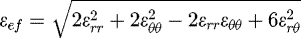
The thermal stress and strain are effective decision making measure for determining the worst or most vulnerable area in terms of the strength and deformation. The effective stress and strain contours are shown in Figures 17 and 18. The equation of effective stress and effective strain in this study is (9) and (10). The contours of Figures 17 and 18 show that the highest amount of effective stress and strain occurs in the fin of row 1, which is due to the higher temperature gradient in this fin than in other fins. It is also observed that the highest amount of effective stress and strain is in the fin base of row 1 at the area C and approximately at zero angle. However, in rows 2, 3 and 4, the highest amount of effective stress and strain at the fin edge the is approximately at an angle of 70 and ‑70 degrees and this is because of the absolute value of the stress as well as the shear strain at the fin edge in rows 2, 3, and 4, which has significant value compared to the maximum tangential stresses at the fin base. The position of the worst place is influenced by this issue. Also, behind the fin of row 4, the effective stress and strain have increased compared to the fins of rows 1, 2 and 3 in the base location and the fin edge which is due to the temperature variations created in it.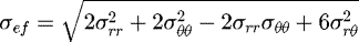 (9)
(9)
 (10)
(10)
 |
Fig. 17 Effective stress contours in the finned tubes bank (inlet flow rate = 2 m/s). |
 |
Fig. 18 Effective strain contours in the finned tubes bank (inlet flow rate = 2 m/s). |
4.5 The comparison of an alone fin under periodic condition and each fin into the bundle of fins
In this section an alone fin under periodic condition is simulated. The simulation of a fin under periodic condition in the streamwise direction had been done by [30]; therefore, same simulation method is used in this paper. The aim of this section is to compare the obtained results from previous sections with the alone fin under periodic condition. Same dimensions of the present fins into the finned-tube bundle are considered for designing of alone fin. The comparison of the obtained results in Figure 19 with Figures 10 and 17 shows that stress and temperature distributions of alone fin (a fin with periodic condition) are similar to fins of 2, 3, and 4 rows but they are different from fin of first row. Moreover, more matching there is between second row fin and alone fin. The location and value of maximum stresses are expressed in Table 4. Also, the maximum value of effective stress and critical location of effective stress are shown in Table 4. As seen, while the location of maximum stresses of alone fin are similar to fins of 2, 3 and 4 rows, the value of stresses are different from each other except for second row. In addition, the CPU time for alone fin was compared with the CPU time of finned-tube bank. The CPU time for alone fin was 240 h while the CPU time for bank of finned tubes was 2 h. Therefore, the running time of bank of finned tubes was faster than running time of the alone fin under periodic condition.
 |
Fig. 19 Temperature and effective Stress Contours (a fin with periodic condition). |
The comparison of stresses (MPa).
4.6 Effect of change shape of the first row fin on heat transfer
Since the maximum amount of effective stress and strain is in fin of row 1, we are looking for a solution to reduce stress in this fin. To achieve this, four types of deformation are first applied to the annular fin of the row 1 as shown in Figure 20, and the efficiency of the fin bundle is calculated in each case. For this purpose, the efficiency of the fin bundle is defined as the equation (11) (the ratio of the Nusselt number to the friction coefficient) and then the efficiency percent is calculated according to the equation (12) and is expressed in Table 5. The results of Table 6 show that the best modes are mode 3 and then mode 1 in terms of the thermal efficiency. In the next section, we examine the effective stresses in these modes and compare it with the 0 mode (reference mode). (11)
(11)
 (12)
(12)
That ai, bi are variables in various states.
 |
Fig. 20 Geometry exchange of the fin of first row. |
Thermal effeciency for various modes.
The comparison of effective stress and strain for two modes 0 and 1.
4.7 Effect of change shape of the first row fin on effective stress and strain
Figure 21 shows the temperature and stress contours of the fin of first-row for both 0 and 3 modes. As can be seen, the shape change of mode 3 increases the effective stress because of increase of the temperature gradient, so this type of shape change is not suitable. Now, considering that mode 1 has the highest value of thermal efficiency after mode 3, we examine the stress in this mode. Figure 22 shows the geometry of the finned-tube bundle with the created shape change in the fin of first row (mode 1). In this figure, rv = 12 mm and rh = 13 mm. The effective stress and strain contours are shown in Figures 23 and 25 for the two modes A (Mode 0) and B (Mode 1). Figures 23 and 25 show that the highest amount of effective stress and strain in both A and B modes is at the fin of row 1, which is due to having higher temperature gradient in this fin than in other fins. Also, you can see in the contours of the effective stress in Figure 23 that the maximum point of the stress in mode A is at the fin base and in mode B is at the fin edge. This is due to the decrease in temperature gradient in the radial direction in area C of the fin at the mode B, as seen in the temperature contours of these two fins in Figure 24. On the other hand, a comparison of the decrease or increase rate of the effective stress and strain of mode B and mode A (zero mode) in Table 6 shows that changing the shape of the tube as elliptical in row 1 causes a significant reduction of the effective stress and strain in the fin of row 1 and a slight increase of the effective stress and strain in other rows. As a result, the shape change of the fin of row 1 is a good way to increase the thermal efficiency and reduce the stress.
 |
Fig. 21 Temperature and effective Stress Contours in the fin of first row for 0 mode and 3 mode. |
 |
Fig. 22 Fin of first row (Mode 1). |
 |
Fig. 23 Effective stress contours in the finned tubes bank for two modes A and B at input speed 2 m/s. |
 |
Fig. 24 Temperature contours in the fin of first row for both A and B modes. |
 |
Fig. 25 Effective strain contours in the finned tubes bank for both A and B modes at input speed 2 m/s. |
5 Conclusion
In this paper, the thermal stresses and strains in a four-row annular finned-tube bundle exposed to the transverse flow were analyzed. The fluid flow was turbulent, and the fins were in line arrangement. The finite volume method and the Transition SST model, along with the SIMPLE algorithm, were used to solve the flow equations using FLUENT software, and the finite element method was used to solve the thermal stress equations in the solid using ANSYS software. Studies have shown that although the maximum temperature difference in the fin bundle is less than 1 K degree, the maximum effective stress and strain, which are 0.67 MPa and 1.36e‑5, respectively, cannot be ignored. It should also be noted that with increasing temperature difference between the fluid and the fin base and because of the asymmetric distribution of temperature, the importance of studying the heat flow on thermal stresses and strains increases. The obtained results of the study on the effect flow on the created strains and stresses in an annular finned-tube bundle are summarized as follows:
-
The highest effective stress and strain appeared in the first row.
-
The temperature gradient, stress, and strain in row 1 were different from other rows.
-
The highest effective stress in the first row occurred in the fin base. In the other rows, they appeared at the edge of the fin. The effective stress and strain were greater in the first and second rows than in the third and fourth rows.
-
The highest effective stresses were observed in area C of row 1 and areas A and B of rows 2, 3 and 4.
-
The highest effective strains for all rows were observed in areas A and B.
-
In area D of rows 1, 2, and 3, the effective stress and strain were relatively low, but in row 4, they were higher than in other rows.
-
In all rows, temperature gradient had a dominant influence on tangential stress and tangential strain.
-
The radial strain of the highest magnitude in row 1 appeared in the base of the fin. In rows 2, 3 and 4, it was observed at the edge of the fin at angles of about 70 and −70 degrees.
-
The tangential stress and strain of the greatest magnitude in row 1 were seen in the base of the fin. In other rows, they appeared at the edge of the fin at angles of about 70 and −70 degrees.
-
The highest absolute value of the stress and shear strain of the fin of row 1 is about 110 and 110 degrees and that of the other fins in rows 2, 3 and 4 is around 70 and −70 degrees at the fin edge.
-
The comparison of alone fin under periodic condition with each fin into the fins bundle showed that more matching there was between alone fin and fin of second row.
Based on all the results, it is clear that it is necessary to take into account the thermal stresses and strains in the design of annular fins.
Also, our examination of the outcomes of geometrical change of tube of first row showed that using elliptical tubes in heat exchangers can be a good solution to reduce stress and increase thermal efficiency.
Nomenclature
English symbols
cp : Specific heat at constant pressure, j/kg k
E : Modulus of elasticity, Pa
h : Convective heat transfer coefficient, W/m2 k
kf : Thermal conductivity, W/mk
kt : Turbulent thermal conductivity, W/mk
r : Radius, m
rb : Inner radius of the fin, m
re : Outer radius of the fin, m
Srr : Radial stress
Sθθ : Tangential stress
Srθ : Shear tress
T : Temperature, K
Ta : Fluid temperature, K
Tb : Temperature at the fin base, K
u : Displacement, m
wt : Fin thickness, m
Greek symbols
α : Surface absorptivity
α* : Thermal expansion coefficient
ε : Surface emissivity
εrr : Radial strain
εθθ : Tangential strain
υ : Poisson's ratio
ρ : Density, kg/m3
μ : Dynamic viscosity, kg/ms
μt : Turbulent viscosity, kg/ms
References
- S. Wu, Analysis on transient thermal stresses in an annular fin, J. Therm. Stress. 20 , 591–615 (1997) [CrossRef] [Google Scholar]
- L.-T. Yu, C.-K. Chen, Application of the hybrid method to the transient thermal stresses response in isotropic annular fins, J. Appl. Mech. 66 , 340–346 (1999) [Google Scholar]
- C.H. Chiu, C.K. Chen, Application of the decomposition method to thermal stresses in isotropic circular fins with temperature-dependent thermal conductivity, Acta Mech. 157 , 147–158 (2002) [Google Scholar]
- I.G. Aksoy, Thermal analysis of annular fins with temperature-dependent thermal properties, Appl. Math. Mech. (English Ed.) 34 , 1349–1360 (2013) [CrossRef] [Google Scholar]
- R. Roy, S. Ghosal, Homotopy perturbation method for the analysis of heat transfer in an annular fin with temperature-dependent thermal conductivity, J. Heat Transfer. 139 , 022001 (2016) [Google Scholar]
- H. Sen Peng, C.L. Chen, Hybrid differential transformation and finite difference method to annular fin with temperature-dependent thermal conductivity, Int. J. Heat Mass Transf. 54 , 2427–2433 (2011) [Google Scholar]
- A. Aziz, The effects of internal heat generation, anisotropy, and base temperature nonuniformity on heat transfer from a two-dimensional rectangular fin, Heat Transf. Eng. 14 , 63–70 (1993) [CrossRef] [Google Scholar]
- W. Lau, C.W. Tan, Errors in one-dimensional heat transfer analysis in straight and annular fins, J. Heat Transfer. 95 , 549 (2010) [Google Scholar]
- A. Mallick, R. Das, Application of simplex search method for predicting unknown parameters in an annular fin subjected to thermal stresses, J. Therm. Stress. 37 , 236–251 (2014) [CrossRef] [Google Scholar]
- M.T. Darvishi, F. Khani, A. Aziz, Numerical investigation for a hyperbolic annular fin with temperature dependent thermal conductivity, Propuls. Power Res. 5 , 55–62 (2016) [CrossRef] [Google Scholar]
- M. Sudheer, G.V. Shanbhag, P. Kumar, S. Somayaji, Finite element analysis of thermal characteristics of annular fins with different profiles, Eng. Appl. Sci. 7 , 750–759 (2012) [Google Scholar]
- A. Campo, A.M. Delgado-Torres, Approximate, analytical procedure for rectangular annular fins by accommodating the Cauchy–Euler equation, Int. J. Heat Mass Transf. 124 , 74–82 (2018) [Google Scholar]
- J.Y. Jang, J.T. Lai, L.C. Liu, The thermal-hydraulic characteristics of staggered circular finned-tube heat exchangers under dry and dehumidifying conditions, Int. J. Heat Mass Transf. 41 , 3321–3337 (1998) [Google Scholar]
- S.B.H.C. Neal, J.A. Hitchcock, A study of the heat transfer process in banks of finned tube in cross flow using a large scale model technique, in Proceeding Third Int. Heat Transf. Conf. , 1966, 290–298, available at https://www.osti.gov/biblio/4224258 (accessed February 26, 2019) [Google Scholar]
- M.S. Mon, U. Gross, Numerical study of fin-spacing effects in annular-finned tube heat exchangers, Int. J. Heat Mass Transf. 47 , 1953–1964 (2004) [Google Scholar]
- H. Bilirgen, S. Dunbar, E.K. Levy, Numerical modeling of finned heat exchangers, Appl. Therm. Eng. 61 , 278–288 (2013) [Google Scholar]
- J.Y. Jang, J.Y. Yang, Experimental and 3-D numerical analysis of the thermal-hydraulic characteristics of elliptic finned-tube heat exchangers, Heat Transf. Eng. 19 , 55–67 (1998) [CrossRef] [Google Scholar]
- X. Hu, A.M. Jacobi, Local heat transfer behavior and its impact on a single-row, annularly finned tube heat exchanger, ASME J. Heat Transf. 115 , 66–74 (1993) [CrossRef] [Google Scholar]
- V.B. Kuntysh, N.N. Stenin, Heat transfer and pressure drop in cross flow through mixed inline-staggered finned tube bundles, Therm. Eng. 40 , 126–129 (1993) [Google Scholar]
- M. Mon, Numerical investigation of air-side heat transfer and pressure drop in circular finned-tube heat exchangers, 2003. http://www.qucosa.de/fileadmin/data/qucosa/documents/2029/dissmon.pdf [Google Scholar]
- H. Shokouhmand, S. Mahjoub, M.R. Salimpour, Constructal design of finned tubes used in air-cooled heat exchangers, J. Mech. Sci. Technol. 28 , 2385–2391 (2014) [CrossRef] [Google Scholar]
- H. Nemati, M. Moghimi, Numerical study of flow over annular-finned tube heat exchangers by different turbulent models, CFD Lett. 6 , 101–112 (2014) [Google Scholar]
- H. Nemati, S. Samivand, Numerical study of flow over annular elliptical finned tube heat exchangers, Arab. J. Sci. Eng. 41 , 4625–4634 (2016) [Google Scholar]
- E.N. Pis'Mennyi, Heat transfer enhancement at tubular transversely finned heating surfaces, Int. J. Heat Mass Transf. 70 , 1050–1063 (2014) [Google Scholar]
- V.B. Kuntysh, N.M. Kuznetsov, Thermal and aerodynamic design of air cooling finned heat exchangers, in: Saint-Petersburg, 1992 [Google Scholar]
- S. Wang, G. Jian, J. Xiao, J. Wen, Z. Zhang, J. Tu, Fluid-thermal-structural analysis and structural optimization of spiralwound heat exchanger, Int. Commun. Heat Mass Transf. 95 , 42–52 (2018) [CrossRef] [Google Scholar]
- L. Zhang, Z. Qian, J. Deng, Y. Yin, Fluid-structure interaction numerical simulation of thermal performance and mechanical property on plate-fins heat exchanger, Heat Mass Transfer. (2015) 10.1007/s00231-015-1507-5 [Google Scholar]
- L. Demirdzic, S. Muzaferija, Numerical method for coupled fluid flow, heat transfer and stress analysis using unstructured moving meshes with cells of arbitrary topology, Comp. Meth. Appl. Mech. Eng. 125 , 235–255 (1995) [CrossRef] [Google Scholar]
- I.T. Alzaharnah, MS. Hashmi, B. Yilbas, Thermal stresses in thick-walled pipes subjected to fully developed laminar flow, J. Mater. Process. Technol. 118 , 50–57 (2001) [CrossRef] [Google Scholar]
- M. Hosseini, A. Hatami, S. Payan, Comparison of the effect of laminar and turbulent flow regimes on thermal stresses and strains in an annular fin, J. Mech. Sci. Technol. 34 , 413–424 (2020) [CrossRef] [Google Scholar]
- El. Hami, Abdelkhalak, B. Radi, Fluid-structure interactions and uncertainties: ansys and fluent tools, John Wiley & Sons, 2017 [Google Scholar]
- Verein Deutscher Ingenieure, VDI- Wärmeübergang, Berechnungsblätter fürden Wärmeübergang, 8. Aufl. Berlin u.a., Springer, 2000 [Google Scholar]
- Th.E. Schmidt, Der Wärmeübergang a Rippenrohre und die Berechnung von Rohrbündel-Wärmeaustauschern, Kältetechnik, Band 15, Heft 12, (1963) [Google Scholar]
Cite this article as: A. Hatami, S. Payan, M. Hosseini, Numerical analysis of thermal stresses and strains of annular finned tube bundle in turbulent flow regime, Mechanics & Industry 21, 601 (2020)
All Tables
All Figures
|
Fig. 1 Annular finned tube bundle (A) X1–X3 plane, (B) X1-X2 plane, (C) a distinct fin. |
| In the text | |
|
Fig. 2 Grid type defined for the fins. |
| In the text | |
|
Fig. 3 Grid type defined for the fluid domain and fin-fluid interface. |
| In the text | |
|
Fig. 4 Geometry of an annular fin having inner radius a and tip radius b. |
| In the text | |
|
Fig. 5 Comparison of temperature values. |
| In the text | |
|
Fig. 6 Comparison of radial stress. |
| In the text | |
|
Fig. 7 Comparison of tangential stress. |
| In the text | |
|
Fig. 8 Comparison of temperature values. |
| In the text | |
|
Fig. 9 Legend of areas and angles. |
| In the text | |
|
Fig. 10 Temperature contours of the fins (inlet flow rate = 2 m/s). |
| In the text | |
|
Fig. 11 Radial stress contours in the finned tubes bank (inlet flow rate = 2 m/s). |
| In the text | |
|
Fig. 12 Tangential stress contours in the finned tubes bank (inlet flow rate = 2 m/s). |
| In the text | |
|
Fig. 13 Shear stress contours in the finned tubes bank (inlet flow rate = 2 m/s). |
| In the text | |
|
Fig. 14 Radial strain contours in the finned tubes bank (inlet flow rate = 2 m/s). |
| In the text | |
|
Fig. 15 Tangential strain contours in the finned tubes bank (inlet flow rate = 2 m/s). |
| In the text | |
|
Fig. 16 Shear strain contours in the finned tubes bank (inlet flow rate=2m/s). |
| In the text | |
|
Fig. 17 Effective stress contours in the finned tubes bank (inlet flow rate = 2 m/s). |
| In the text | |
|
Fig. 18 Effective strain contours in the finned tubes bank (inlet flow rate = 2 m/s). |
| In the text | |
|
Fig. 19 Temperature and effective Stress Contours (a fin with periodic condition). |
| In the text | |
|
Fig. 20 Geometry exchange of the fin of first row. |
| In the text | |
|
Fig. 21 Temperature and effective Stress Contours in the fin of first row for 0 mode and 3 mode. |
| In the text | |
|
Fig. 22 Fin of first row (Mode 1). |
| In the text | |
|
Fig. 23 Effective stress contours in the finned tubes bank for two modes A and B at input speed 2 m/s. |
| In the text | |
|
Fig. 24 Temperature contours in the fin of first row for both A and B modes. |
| In the text | |
|
Fig. 25 Effective strain contours in the finned tubes bank for both A and B modes at input speed 2 m/s. |
| In the text | |
Current usage metrics show cumulative count of Article Views (full-text article views including HTML views, PDF and ePub downloads, according to the available data) and Abstracts Views on Vision4Press platform.
Data correspond to usage on the plateform after 2015. The current usage metrics is available 48-96 hours after online publication and is updated daily on week days.
Initial download of the metrics may take a while.