© Q. Serra and E. Florentin, Published by EDP Sciences, 2023

1 Introduction

Dealing with uncertainties has been the subject of intense research recently. The output of deterministic codes may indeed differ from the reality because of several factors: (1) inadequacy between mathematical model and reality (e.g. differences in material properties, boundary conditions, loading, etc.) in both reality and numerical simulation, and (2) numerical errors due to space or time discretization, for example. Numerical methods, whether for space or time discretization, are well-mastered today, and error estimates can be obtained even in commercial codes. Therefore, researchers have focused on the development of stochastic methods, to generalize deterministic codes and address parametric uncertainties in the model, such as material uncertainty or geometrical uncertainty in processes. Such algorithms have numerous applications, including risk management, optimization, and robust design [1,2]. The biggest drawback of stochastic problems is the significant numerical cost required to explore the stochastic space. A review of several stochastic methods has been proposed in [3,4].

Monte Carlo (MC) simulation [5] is often used as a reference. It is an approximate method for assessing some probabilistic moments of the quantity of interest. The advantage is that it does not require any complex computer code dedicated to stochastic problems, but its drawback is slow convergence. Consequently, it entails a significant computational cost. Variance reduction techniques have been developed to achieve better convergence [6]. Last, but not least, this method does not allow for the generation of a surrogate. Therefore, it is not possible to approximate the quantity of interest outside of the numerical experimental design (NED). Several strategies have been developed to address this computational cost.

Perturbation methods are based on a Taylor series expansion around the mean value of parameters. They are limited to cases involving small variations of a smooth random field around its mean value. A wide range of other metamodeling techniques has been proposed, for example Radial Basis Functions (e.g. [7,8]), kriging (e.g. among many, [9]), Support Vector Machines (e.g. [10]), or coupled approaches (e.g. [11,12]). We focus solely on polynomial chaos, even though all of the content presented below can be easily transposed to other surrogates. The polynomial chaos (PC) expansion is a spectral method, it consists in an approximation of the stochastic response in the space spanned by a finite basis of orthonormal polynomials. It is based on the Homogeneous Chaos theory initiated by Wiener [13] and later extended by others [14,15]. An intrusive strategy is employed when the PC expansion is used in conjunction with a Galerkin approach (see for example [16,17]). However, this results in a significant computational cost and the need to write a dedicated program. A second strategy is non-intrusive, it consists in computing the coefficients of the expansion as the projection of the Quantity of Interest (QoI) on the space spanned by the polynomial basis. Two approaches are classically used. The first one is called Non-Intrusive Spectral Projection [18], where the projection is computed numerically using a quadrature rule. The second one relies on linear regression to compute the best coefficients (in a least square sense) of the PC expansion.

To assess the accuracy of the PC expansion and control the error, which represents the difference between the response and its projection using the chosen polynomials, we require error estimates. Several studies have explored the a priori convergence behavior of the PC expansion [19,20]. In the projection approach, the a priori error bound is determined by the Koksma–Hlawka inequality, and it is directly influenced by the choice of sampling points.

In regression based framework, various authors have recently developed different strategies to build adaptive PC expansion. These strategies incorporate a posteriori error control based on factors like the variance decrease rate [21], the residual decrease rate [22,23], or scalar values such as the R² regression coefficient or the Leave One Out error [24–26]. However, while these indicators offer valuable insights, these indicators provide only qualitative information on the meta-model’s quality, necessitating users to set tolerance values arbitrarily. An alternative approach, commonly used in statistical learning, is to measure the mean square error on an empirical test dataset. In Dao et al. [27], the authors proposed such an approach, but the error was derived from a residual based problem. However, using a small dataset leads to a non-robust estimate of the mean square error, while employing a large size of testing datasets leads to prohibitive computation costs. Another drawback of a mean square estimate is that the error estimate is global on stochastic domain, making it impossible to assess the local error value at a given arbitrary point.

Another approach is to introduce a dual problem to estimate the local error (see [28,29] for details). It makes it possible to estimate the local error with a good accuracy but requires to define the dual problem associated with the chosen Qol. The Qol must depend linearly on the displacement. In addition to the necessary theoretical developments, this method generates additional simulation costs which are far from negligible. The objective of this paper is to define a method that is simple to implement and has a reasonable cost (like the MSE and LOO methods) for local quality estimation (like the dual methods).

While Dao et al. explored transient dynamics in their study [27], our focus in this paper is on structural vibrations. This type of problem is quite common, as uncertainties often manifest themselves in the mid-frequency range. Consequently, there's a substantial body of scientific work in this area (e.g., [30]). An earlier study by [16] has shown that a frequency-frozen intrusive polynomial chaos expansion does not converge quickly, and the convergence rate depends on the parity of the polynomial order. Aitken’s sequence has been proposed in [16] to improve the rate of convergence of PC expansion, but once again the convergence is slow. Two different approaches have resulted in a better match between the polynomial chaos surrogate and the reference model. The first approach uses a PC expansion, not on the physical unknown but on the modal parameters of the system. The second one consists in adding supervision on the spectrum of the output, using Pade expansion [17]. However, in these articles the reference was always provided, and the MSE and the LOO were taken as error estimates.

In real-world industrial scenarios, the computational cost limits the use of PC expansions to lower polynomial orders. Hence, accurate quantitative error estimates are crucial to assess the metamodel’s validity. However, many existing literature-derived error estimates fall short when dealing with small Numerical Experimental Designs (NEDs). Furthermore, the reference is often unknown beyond the training points. In this paper, we propose employing a polynomial chaos expansion to solve a residual-based stochastic equation associated with the reference problem. Our aim is to assess the error resulting from the PC expansion efficiently, not just the global mean square error, but also the local error at specific test points. Additionally, we validate our approach by comparing it to the reference error value, even though, in practical industrial cases, a reference value for validation might not be accessible.

Another crucial aspect to consider while reading this document is that we are primarily interested in quantifying the error attributed to the metamodel. Typically, the error stemming from stochastic metamodeling techniques is much larger than the error from conventional discretization methods, such as finite difference for time discretization or finite elements for space discretization. Therefore, we don’t need to employ an overly precise method for the initial metamodel. Instead, our goal here is to develop efficient error estimation strategies for such a coarse PC surrogate.

The manuscript is structured as follows. In Section 2, we provide a theoretical overview of PC expansion applied to structural vibrations. In Section 2.4, we present a practical example that showcases a three-degree-of-freedom (3-DOF) problem. Despite its apparent simplicity, this academic system serves as a representative model for various industrial challenges related to mechanical vibrations. Section 3 delves into the details of our error estimation strategy. The primary concept introduced in this article is that we can estimate the error using a non-intrusive polynomial chaos approach, and we present two variants of this approach. The first variant involves straightforward error interpolation, while the second variant employs a modal basis decomposition of the approximation, offering a highly cost-effective error estimation tool. This tool enables precise control of mechanical vibration problems with minimal additional expenses. In Section 4, we examine and analyze the results using the common thread example.

2 Structural vibrations and polynomial chaos expansion

2.1 Notations

Scalar numbers and functions are written in a normal font, e.g. x, y, a, b, ω. Vectors are written with an underlined font, e.g. $\underset{\_}{Fx}$, $\underset{\_}{R}$. Matrices are written roman bold symbol font, e.g. K, M, ϕ. For sake of clarity, Tables A.1 and A.2 in appendix A present the list and description of every variable used in the paper.

2.2 Structural vibrations with parametric uncertainties

Assuming that the problem has been discretized in a finite number (n) of discrete unknowns, the dynamic equilibrium of a linear mechanical system can be written for each pulsation ω as:

$$\left[-{\omega }^{2}M\text{\hspace{0.17em}+\hspace{0.17em}i}\omega C+K\right]\underset{\_}{x}\left(\omega \right)=\underset{\_}{F}\left(\omega \right)$$(1)

where M, C and K are respectively the (n × n) mass matrix, damping matrix and stiffness matrix of the discrete system, $\underset{\_}{x}$ is the vector of nodal displacements, which are unknown, $\underset{\_}{F}$ is the vector of nodal loads.

This problem can be solved in physical coordinates, but often, the transformation into modal coordinates is preferred. This reduces the numerical cost, especially for finite element studies in the low frequency range. It is also very useful for sub-structuring complex systems.

Structural modes (${\omega }_i,{\underset{\_}{\varphi }}_i$) are defined by the classical relations:

$$K{\underset{\_}{\varphi }}_i={\omega }_i^{2}M{\underset{\_}{\varphi }}_i$$(2)

and usually the n_m eigenvectors are normalized with respect to the mass matrix, so the modal matrix $\varphi =\left[{\underset{\_}{\varphi }}_1\cdots {\underset{\_}{\varphi }}_{n_m}\right]$ is such that:

$$\begin{array}{cc}{\varphi }^{T}M\varphi =Id,& {\varphi }^{T}K\varphi =diag\left({\omega }_i^2\right)\end{array}$$(3)

The Basile’s hypothesis states that the damping matrix is also diagonalized in the modal basis, several possibilities exist to define this matrix: Rayleigh damping, hysteretic damping or viscous damping hypothesis can be classically found. We consider here the hypothesis of an hysteretic damping iωC = iηK. Once the modal characteristics of the system are known, the complex physical response $\underset{\_}{x}$ can be obtained as a linear expansion on the modes:

$$\underset{\_}{x}=\varphi \underset{\_}{Q}={\displaystyle \sum _{i=1}^{n_m}{Q}_i\left(\omega \right){\underset{\_}{\varphi }}_i}$$(4)

where

$$\begin{array}{cc}\forall i\in \left\{1,\dots ,n_m\right\},& Q_i\left(\omega \right)=\frac{{\underset{\_}{Q}}_i^T\underset{\_}{F}\left(\omega \right)}{{\omega }_i^2\left(1+\text{i}\eta \right)-{\omega }^2}\end{array}$$(5)

The nature of the vibratory response reveals that high-frequency modes exhibit relatively low amplitudes in the modal expansion. As a result, engineers often employ a truncation criterion based on the eigenfrequencies to eliminate these high-frequency modes from the expansion. This leads to a significantly smaller number of modes compared to the number of degrees of freedom in finite element analysis. In certain cases, a static correction technique is employed to account for the contribution of high-frequency modes. In situations involving parametric uncertainties, some values within the matrices and the external load vector may be subject to randomness. Consequently, the dynamic response vector $\underset{\_}{x}$, along with the eigenmodes, eigenvalues, and eigenvectors, becomes a random variable. Various examples can be found in the literature, such as the one mentioned in [31], which serves as the basis for our common thread example discussed in Section 2.4.

2.3 Polynomial chaos approximation

A polynomial chaos approximation of a random process with finite second-order moments is a mathematical model obtained by the approximation of the exact random process in the space spanned by a family of polynomials.

Generally, in vibration problems, the quantity of interest is the vector of displacements at each frequency. This quantity of interest can be obtained for an arbitrary realization of the random input parameters as the result of a reference model ℳ applied at pulsation ω to the normalized random input variables $\underset{\_}{\xi }$, by:

$$\underset{\_}{x}\left(\underset{\_}{\xi },\omega \right)=ℳ\left(\underset{\_}{\xi },\omega \right)$$(6)

For any realization of the vector of input parameters $\underset{\_}{\xi }$, the QoI is computed approximately using a linear combination of polynomials ${\underset{\_}{x}}_{PC}$ such as:

$$\underset{\_}{x}\left(\underset{\_}{\xi },\omega \right)\approx \underset{\_}{x}{}_{PC}\left(\underset{\_}{\xi },\omega \right)={\displaystyle \sum _{j=1}^{n_{PC}}{\underset{\_}{X}}_j}\left(\omega \right){\text{Ψ}}_j\left(\underset{\_}{\xi }\right)$$(7)

where Ψ_j are the chaos polynomials and ${\underset{\_}{X}}_j$ are the n_PC chaos coefficients. While numerous infinite families can theoretically represent the random process, practical considerations necessitate using a finite family. Therefore, the choice of the polynomial family directly impacts the convergence of the expansion, as described in equation (7). An optimal choice of the polynomial family depending on the distribution of the random input parameter $\underset{\_}{\xi }$ is provided in [14].

Due to the hypothesis of uniform distributions, we consider here Legendre polynomials.

The regression approach is used in this article to evaluate the chaos coefficients ${\underset{\_}{X}}_j$. It consists in searching an optimal set of chaos coefficients ${\underset{\_}{X}}_j$ in the least square sense:

$$\begin{array}{l}\left\{{\underset{\_}{X}}_1\left(\omega \right),\dots ,{\underset{\_}{X}}_{n{}_{PC}}\left(\omega \right)\right\}\hfill \\ =\underset{\left\{{\underset{\_}{X}}_1\left(\omega \right),\dots ,{\underset{\_}{X}}_{n{}_{PC}}\left(\omega \right)\right\}}{\text{argmin}}\left(\frac{1}{Q}{\displaystyle \sum _{q=1}^Q\left|\underset{\_}{x}\left({\underset{\_}{\xi }}_q,\omega \right)-{{\displaystyle \sum _{j=1}^{n_{PC}}{\underset{\_}{X}}_j\left(\omega \right){\text{Ψ}}_j\left({\underset{\_}{\xi }}_q\right)}}^2\right|}\right)\hfill \end{array}$$(8)

where ${\underset{\_}{\xi }}_1,{\underset{\_}{\xi }}_1,\dots ,{\underset{\_}{\xi }}_Q$ are the Q realizations of the input parameters and |●| is the modulus of a complex number.

If we introduce the matrix Ψ = (Ψqj)_{qϵ{1..Q},jϵ{1..N}} with Ψqj = Ψj(${\underset{\_}{\xi }}_q$)), then the solution can be obtained by computing the Moore-Penrose pseudo-inverse of Ψ denoted Ψ⁺:

$${\Psi }^{+}={\left({\Psi }^T\Psi \right)}^{-1}{\Psi }^T$$(9)

The number Q of sampling points ${\underset{\_}{\xi }}_q$ should be at least equal to the number of polynomials. The robustness of the estimation of the chaos coefficients increases with this number, but so does the numerical cost. Writing r the number of random input parameters and p the maximal order for each polynomial, a full tensor product of mono-variate polynomials leads to n_PC = (p + 1)^r polynomials. For this reason polynomial chaos suffers from the curse of dimensionality. Another problem arises from the condition number of the Fisher matrix Ψ^T Ψ, which depends on the choice of the polynomials but also on the choices of the sampling points.

In the literature, the sampling points are classically chosen among Gauss collocation points, or with (quasi-)random sequences [32]. A Latin Hypercube sampling (LHS), using Q = k.n_PC simulations (with k = 2, 3 or 4), is usually considered. This choice is a good compromise between robustness of least square minimization, numerical cost, and ease in programming for industrial codes or adaptive schemes.

Sparse truncation techniques [33] can be used to reduce computational burden. Here, we only consider the classical truncation scheme, which conduces to a reduced number of polynomials:

$$n_{PC}=\frac{\left(p+r\right)!}{p!r!}.$$(10)

These techniques are typically used with adaptive algorithms, which need efficient error measures. The matter of measuring errors holds significant importance when dealing with these sparse models. It’s essential to clarify that in this work, our primary goal is not to reduce the cost of the surrogate model. Instead, our objective is to predict the approximation error. Therefore, we’re not seeking to determine the optimal choices for factors like polynomials or sampling methods. Instead, we will rely on conventional PC approaches.

2.4 Illustrative example

In this section, we present some results demonstrating the application of PC approaches to vibration problems.

We consider here the following stochastic problem with three degrees of freedom n = 3, illustrated in Figure 1, where the quantity of interest is the random vector:

$$\underset{\_}{x}\left(t\right)={\left[x_1,x_2,x_3\right]}^T$$(11)

This simple system can be understood as a 3-mode

reduction of a real, continuous,3d, mechanical structure. The mass and stiffness matrices are given by:

$$\begin{array}{l}M=\left[\begin{array}{ccc}{m}_1& 0& 0\\ 0& m_2& 0\\ 0& 0& m_3\end{array}\right],\hfill \\ K=\left[\begin{array}{ccc}{k}_1+k_4+k_6& -k_4& -k_6\\ -k_4& k_2+k_4+k_5& -k_5\\ -k_6& -k_5& k_3+k_5+k_6\end{array}\right]\hfill \end{array}$$(12)

The values of the stiffness k_i vary randomly, each random stiffness follows a uniform distribution of mean k_i = 1 N/m for i = 1…5, and equal to 3N/m for k₆. The standard deviation of each random stiffness is σ_k = 0.15 N/m. The three masses are defined as m_i = 1 (deterministic). The load, applied to the first dof, is equal to 1N at every frequency, its amplitude follows a uniform distribution with a standard deviation equal to 0.15 N. A deterministic hysteretic damping η = 0.01 is used to compute the frequency spectrum. Therefore, the stochastic problem has 7 random variables.

The reference is computed with a Monte Carlo approach using a random sampling of 10⁵ samples, this number being chosen to reach convergence. Finally the x-axis is transformed into a non-dimensional axis using as a reference pulsation ${\omega }_0=\sqrt{\text{mean\hspace{0.17em}}\left(k_1\right)/m_1}$.

We only present results for x₁, dof number 1, but similar results are obtained for other dofs.

Figure 2a displays the mean and the envelope (95% confidence interval) of the response obtained by the reference computation (Monte Carlo) and by a first-order PC approximation. To assess the method’s accuracy, we propose to plot in Figure 2b the residue of the PC approximation. This residue is defined by:

$$\underset{\_}{R}\left(\underset{\_}{\xi },\omega \right)=\underset{\_}{F}\left(\underset{\_}{\xi }\right)-\left[-{\omega }^{2}M+K\left(\underset{\_}{\xi }\right)\left(1+\text{i}\eta \right)\right]{\underset{\_}{x}}_{PC}\left(\underset{\_}{\xi },\omega \right)$$(13)

This residue can be evaluated very quickly, the numerical cost coming only from the large amount of snapshots, and from the need to evaluate the system matrices for each random realization. We recall that the load applied on the first dof is such that F₁ = 1N, so that 10 log₁₀(F₁) = 0. Consequently, the residue can be considered as small if 10 log₁₀(|R₁|) < −10.

The same figures are plotted on Figure 3 for a fourth-order PC expansion.

It can be observed that PC expansions lead to good prediction of the stochastic field, but only far from the resonance pulsations. The prediction becomes globally closer to the reference when the approximation order increases. However, in the vicinity of resonance frequencies, an increase of the order increases slightly the quality of the approximation, but the residual stays at a high level. This occurs because the eigenvalue is stochastic, which means that the resonance peak can either be lower or higher than the load pulsation. This results in a non-smooth function that is challenging to represent accurately using polynomials. Furthermore, looking to both displacement and residual results makes it possible to conclude that the residual is high when the loading frequency belongs to the interval of possible eigenfrequencies. Thus, as an intermediate conclusion for this part, we can state that a classical PC approach should only be used for frequencies which do not belong to the confidence interval of the stochastic eigenfrequencies. Thus, when applying PC expansion to vibrations problems, the main difficulty for the user lies in evaluating the metamodel’s quality. This evaluation is the goal of the next section.

Fig. 1 3-dof system considered in the study, issued from [31].

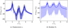Fig. 2 Mean and 95%-confidence interval envelope of the displacement x1 and of the residual R1 on reference (105) points for a 1st-order PC approximation. Black line and grey envelope: reference results.

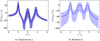Fig. 3 Mean and 95%-confidence interval envelop of the displacement x1 and of the residual R1 on reference (105 ) points for a 4th-order PC approximation. Black line and grey envelope: reference results.

3 A posteriori estimation of the error

A posteriori estimation of the approximation error is of main importance in industrial cases, because the Monte Carlo approach is not computationally affordable, and the residual does only provide a qualitative information on the accuracy of the surrogate. The idea we defend in this work lies in the fact that every numerical model should be presented with the associated quality level. In this part we will recall classical a posteriori estimates. It will be shown that they are limited in their use and in their ability to catch the error. Another original estimation strategy will be proposed.

3.1 Literature survey

Using ${\underset{\_}{x}}_{PC}$ as an approximation of $\underset{\_}{x}$ following equation (7) leads to an error defined as:

$$\underset{\_}{e}=\underset{\_}{x}-{\underset{\_}{x}}_{PC}$$(14)

A measure of the error, called “generalization error” or Mean Square Error MSE, can be defined:

$$\underset{\_}{\text{MSE}}=E\left[{\left|e\right|}^2\right]$$(15)

This measure takes into account the error on the mean as well as the error on the variance. However it cannot be computed directly. As a consequence, several error estimates have been developed in the literature to estimate this error with a reasonable cost.

3.1.1 The empirical error on training dataset

The Empirical Error on training dataset is a measure of the residue of the least square minimization equation (8). It approximates the empirical error using the different Q sampling points defined in the PC approximation. The empirical error ${\underset{\_}{\text{MSE}}}_{train}$ is computed at a very low cost using:

$${\underset{\_}{\text{MSE}}}_{train}=\frac{1}{Q}{\displaystyle \sum _{q=1}^Q{\left|\underset{\_}{x}\left({\underset{\_}{\xi }}_q\right)-{\underset{\_}{x}}_{PC}\left({\xi }_q\right)\right|}^2=}\frac{1}{Q}{\left|\underset{\_}{e}\left({\underset{\_}{\xi }}_q\right)\right|}^2$$(16)

It can be remarked here that the regression approach of the PC naturally minimizes the empirical error so that this measure can dramatically underestimate the actual level of error. This estimate can also be seen as a coarse Monte Carlo approximation of MSE.

3.1.2 The Leave One Out (LOO) error

The LOO error [34–36] is a measure of the error derived from cross-validation techniques [37]. Considering first a set of Q deterministic samples, it is possible to take Q – 1 samples arbitrarily – that is a set {1,…,Q}\q – and to derive the associated PC expansion: ${\underset{\_}{x}}_{PC}^{\left(\backslash q\right)}$. Instead of this bootstrap approach, Blatman uses in [24] the direct expression :

$$\underset{\_}{\text{LOO}}=\frac{1}{Q}{\displaystyle \sum _{q=1}^Q\frac{{\left|e\left({\underset{\_}{\xi }}_q\right)\right|}^2}{h_q^2}}$$(17)

where h_q are the diagonal terms of the matrix : H = Id – ΨΨ⁺.

The interest of $\underset{\_}{\text{LOO}}$ and ${\underset{\_}{\text{MSE}}}_{train}$ is that their calculation is based only on the values of the QoI in the training dataset, so the numerical cost is very low. However, they only provide qualitative information on the level of error, as it will be illustrated in the next section. An arbitrary tolerance value has to be fixed to evaluate if the PC expansion approximates the random variable correctly.

3.1.3 The empirical error on a (coarse) testing dataset

A third measure is very classical in statistical learning, for example machine learning. It is another empirical measure, based on a coarse Monte-Carlo method. One can remark that the empirical error based on the training dataset (values used to compute the surrogate) is minimal, because the surrogate coefficients are computed through a least-square minimization of this empirical error. So, one can think that these points are not appropriate to evaluate the error. The idea is to measure an empirical error on arbitrary random points in the stochastic space, different from the training points. The cost is much larger, because the exact response of the QoI is needed on the testing dataset. In typical applications the following recipe is often applied: 70% of the sampling points is affected to training, and 30% is affected to tests. This way of measuring the error is more costly, but leads to error levels much more realistic than with the empirical error on training dataset. However, the inherent question concerns the choice of the sampling points, and the consequences of this choice on the variability of the error estimate. Furthermore, using a small amount of sampling points for error estimation may be quite efficient for measuring the mean square error, but it is generally not optimal to evaluate the distribution of the error, typically the histogram and the variance.

In summary, MSE on training data is very fast to compute but suffers in quality. The quality of the prediction can be improved using testing points at the price of a huge numerical cost. Between the two models, LOO is very fast, and is considered as reference in literature. All of the three mentioned methods have the same drawback. They only provide a global indicator, the mean square value over the stochastic space. Neither do they provide the distribution of the error.

The idea developed in this article consists of building a low cost surrogate for the random variable “error” itself, so that each moment of the error can be evaluated, in an approximate way, at a low numerical cost. In particular, the mean, the variance, and the histogram of the PC surrogate of the error can be computed efficiently. Such local surrogate is of great interest.

3.2 Strategy

Introducing the error $\underset{\_}{e}$ defined in equation (14) into equation (1), the problem can be written:

$$\left[-{\omega }^{2}M\left(\underset{\_}{\xi }\right)+\text{i}\omega C\left(\underset{\_}{\xi }\right)+K\left(\underset{\_}{\xi }\right)\right]\underset{\_}{e}\left(\underset{\_}{\xi },\omega \right)=\underset{\_}{R}\left(\underset{\_}{\xi },\omega \right)$$(18)

where, $\underset{\_}{R}$ is the residue associated to the PC approximated solution of the dynamic equilibrium, defined in equation (13).

Therefore, two reasons explain why the error may be larger at some frequencies. The first one is that the form of the equation being similar, the error amplitude may become very important in the vicinity of the eigenfrequencies. The second one comes from the load term, the spectrum of the error increasing with the spectrum of the residual.

The original idea presented in this paper consists of using another PC expansion to solve for equation (18). More explicitly, in literature, error is typically measured at some points (so its exact value is known there), but the computation of the MSE is made by numerical integration, which is approximate, the integral being computed by a weighted sum (Monte Carlo, ${\underset{\_}{\text{MSE}}}_{train}$, ${\underset{\_}{\text{MSE}}}_{test}$, quadrature rules can be seen like this). Each error measurement needs the evaluation of the reference solution, so due to the computational burden only a few points are available. The resulting MSE estimate may be far from the reality.

On the contrary, we propose in this paper to take advantage from PC expansion by using reference testing points to derive a surface response surrogate of the error. The MSE of the error surrogate can then be computed exactly at a low numerical cost. The consequence of the approach is that it makes it possible to estimate the error random variable itself, and not only its mean square value, giving access to other interesting properties, such as the local (in stochastic domain) behaviour of the error.

The key point is to solve correctly equation (18). Indeed, the numerical strategy used to solve this error problem governs the quality and the efficiency of the error estimate. We propose three different numerical strategies, based on polynomial chaos:

1. a PC surrogate of error (PCe).

2. a Modal Basis PC surrogate of error (MbPCe).

3. a One-mode Reduced Modal Basis PC surrogate of error (OR-MbPCe).

The numerical strategy PCe is presented in Section 3.2.1; MB-PCe is presented in Section 3.2.2 and its variant OR-MbPCe in Section 3.2.3.

In the following, notations for the construction of the error surrogate will be kept the same than from the PC surrogate of the displacement, except that for a e-superscript which will be used for the construction of the PC expansion of the error when needed.

3.2.1 PC surrogate of error (PCe)

In this approach the user has to fix a priori the PC expansion order p^e of the resolution of the error problem equation (18), and the set of the Q^e sampling points. Using this sampling of error measurements, the PC expansion of the error takes the form:

$$\underset{\_}{e}\left(\underset{\_}{\xi },\omega \right)\approx {\underset{\_}{e}}_{PC}\left(\underset{\_}{\xi },\omega \right)={\displaystyle \sum _{i=1}^{n_{PC}^e}\underset{\_}{E_i}\left(\omega \right){\text{Ψ}}_i\left(\underset{\_}{\xi }\right)}$$(19)

The first interest of the PC expansion is that the error surrogate is a local estimate in the stochastic space. The second interest is that, once the local approximation is known, it is very easy to have a global value on the stochastic space. In particular, due to the choice of an orthonormal basis, the MSE can be approximated analytically:

$$\underset{\_}{\text{MSE}}\approx {\underset{\_}{\text{MSE}}}_{PC}=E\left[{\left|{\underset{\_}{e}}_{PC}\right|}^2\right]={\displaystyle \sum _{i=1}^{n_{PC}^e}{\left|{\underset{\_}{E}}_i\left(\omega \right)\right|}^2}$$(20)

For another choice of polynomial basis, one could have performed a Monte-Carlo estimate of ${\underset{\_}{\text{MSE}}}_{PC}$, but this is easy because the expression of the error surrogate is analytic.

The question concerning the optimization of the localization of the sampling points for the error problem will not be investigated in the present paper. Although many different sampling strategies can be used, we will only consider a classical Latin hypercube sampling, which lead to robust results.

As observed in Section 2.4, the PC expansion generally yields poor results in the proximity of resonances, thus leading to significant disparities between the actual error level and the predicted error level. To address this issue, in the following section, we propose the application of a Modal Basis PC approach for handling the error problem.

3.2.2 Modal Basis PC surrogate of error (MB-PCe)

The idea behind Modal Basis PC expansion is to use the physical properties of the system. Instead of taking a PC approximation of the error, a PC approximation of the eigenvectors and eigenvalues is computed. Ghienne and Blanze [31] proposed instead a Taylor based approach to evaluate the approximation of the random eigenvectors at the current sampling point. The method allows us to derive the same results, but the real challenge lies in calculating the derivatives of the eigenmodes with respect to the random parameters.

The total error is subsequently evaluated using a Monte Carlo approach using these approximations to fasten up the computation.

Let us first compute ${\underset{\_}{\varphi }}_{i,PC}$, polynomial chaos approximations of the random eigenvectors. They can be written as a linear combination of several snapshots of eigenvectors, and each of the components of the expansion can also be written as a linear combination of deterministic eigenvectors ${\underset{\_}{\overline{\varphi }}}_k$:

$$\begin{array}{l}\forall i\in \left\{1,\dots ,n_m\right\},\hfill \\ {\underset{\_}{\varphi }}_{i,PC}\left(\underset{\_}{\xi }\right)={\displaystyle \sum _{j=1}^{n_{PC}}{\underset{\_}{\text{Φ}}}_{ij}{\text{Ψ}}_j\left(\underset{\_}{\xi }\right)={\displaystyle \sum _{j=1}^{n_{PC}}{\displaystyle \sum _{k=1}^{n_m}{\lambda }_{ijk}{\underset{\_}{\overline{\varphi }}}_k{\text{Ψ}}_j\left(\underset{\_}{\xi }\right),}}}\hfill \end{array}$$(21)

Let us now define the approximated generalized mass matrix $\tilde{M}=\left({\tilde{m}}_{ij}\right)$ and stiffness matrix $\tilde{K}=\left({\tilde{k}}_{ij}\right)$ by:

$$\begin{array}{ll}\forall \left(i,j\right)\in {\left\{1,\dots ,n_m\right\}}^2,\hfill & {\tilde{m}}_{ij}={\underset{\_}{\varphi }}_{i,PC}{\left(\underset{\_}{\xi }\right)}^{T}M\left(\underset{\_}{\xi }\right){\underset{\_}{\varphi }}_{j,PC}\left(\underset{\_}{\xi }\right)\hfill \\ \forall \left(i,j\right)\in {\left\{1,\dots ,n_m\right\}}^2,\hfill & {\tilde{k}}_{ij}={\underset{\_}{\varphi }}_{i,PC}{\left(\underset{\_}{\xi }\right)}^{T}M\left(\underset{\_}{\xi }\right){\underset{\_}{\varphi }}_{j,PC}\left(\underset{\_}{\xi }\right)\hfill \end{array}$$(22)

These matrices correspond to the projection of the random matrices K and M on the space spanned by the approximated eigenvectors ${\underset{\_}{\varphi }}_{i,PC}$. Thus these matrices are not diagonal. It is still possible to seek the solution by taking into consideration the off-diagonal terms of the generalized mass and stiffness matrices, but the problem becomes as complex as the initial problem equation (18), with full matrices to invert instead of sparse matrices. Thus, it is not interesting from a computational point of view.

By making the diagonal approximation of the generalized matrices, the error at pulsation ω can be evaluated

as $\underset{\_}{e}\approx {\underset{\_}{e}}_{MbPC}$ with the following expression:

$${\underset{\_}{e}}_{MbPC}\left(\underset{\_}{\xi },\omega \right)={\displaystyle \sum _{i=1}^{n_m}\frac{{\underset{\_}{\varphi }}_{i,PC}{\left(\underset{\_}{\xi }\right)}^T\underset{\_}{R}\left(\underset{\_}{\xi },\omega \right)}{{\tilde{k}}_{ii}\left(1+\text{i}\eta \right)-{\omega }^2{\tilde{m}}_{ii}}{\underset{\_}{\varphi }}_{i,PC}\left(\underset{\_}{\xi }\right)}$$(23)

The expression equation (23) can be evaluated very quickly once the eigenvalue approximations are known, because equation (23) is analytic and does not imply any linear system to solve, so a Monte Carlo approach can be used.

Once again, a key point will be the influence of the choice of the order and of the sampling for the error PC expansion, relatively to the parameters chosen for the displacement metamodel. However, as we will see in Section 4.3, given the substantially different resolution strategies employed, there are fewer couplings between the parameters of the two surrogates.

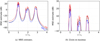Fig. 4 MSE estimates for a 1st-order PC surrogate (plot in dB). Black: reference; blue: MSEtrain; red: LOO.

3.2.3 One-mode reduced modal basis PC surrogate of error (OR-MB-PCe)

This part is a model reduction approach for the MbPCe strategy.

As it was observed in the beginning of this study, classical PC expansion often fails in the vicinity of the eigenfrequencies. Furthermore, the error equation equation (18) shows that the error can be very large in these frequency bands because eigenfrequencies of the system are also eigenfrequencies of the error. So, a good quality estimate is observed by looking at the error level at the resonance peaks. To reduce the amount of modes, which could be high in an industrial context, we propose to select only the modal contribution of the modes belonging to the frequency band of interest. This leads to a huge reduction of memory needs and time to compute the eigenvectors (only one eigenvector to find) and to post-process the error. The drawback lies in the eventual coupling between the modes having the same eigenfrequencies or when modes are coupled by damping effects.

For example, let us say we are interested by the amplitude of the error around the pulsation ω_j, where j corresponds to the j – th mode, then a one-mode truncation of the error modal expansion equation (23) would be:

$${\underset{\_}{e}}_{OR-MbPC}^{\left(j\right)}\left(\underset{\_}{\xi },\omega \right)=\frac{{\underset{\_}{\varphi }}_{j,PC}{\left(\underset{\_}{\xi }\right)}^T\underset{\_}{R}\left(\underset{\_}{\xi },\omega \right)}{{\tilde{k}}_{jj}\left(1+\text{i}\eta \right)-{\omega }^2{\tilde{m}}_{jj}}{\underset{\_}{\varphi }}_{j,PC}\left(\underset{\_}{\xi }\right)$$(24)

Of course, a subset of modes could have been considered in the case of modes having similar eigenfrequencies, we consider here one mode expansion because of the empirical distribution of the eigenfrequencies (cf. Fig. 6). Finally, the approximation of the MSE is obtained by computing the Monte-Carlo mean of the square of the error estimate, this computation being fast because of the analytic nature of equation (24).

4 Numerical results

In this section, we apply the error estimation strategies to the PC surrogate depicted in Section 2.4, corresponding to the mechanical system illustrated in Figure 1. We consider a low cost PC surrogate obtained by taking classical rules of thumb for the amount of points and a first order PC expansion of the displacement (the surrogate depicted in Fig. 2). The idea behind this choice, which is obviously not the best, is that our strategy does not depend on the displacement surrogate. Moreover, for industrial problems, simple surrogates are typically tested first; the key point is thus to know how far from the reality these coarse surrogates are. For sake of conciseness, results are only presented for the first degree of freedom.

4.1 LOO and training MSE

Figure 4 presents the classical error estimates presented in the previous section: MSE on training data and LOO. The exact MSE is approximated by the empirical MSE on testing points (10⁵ samples). We can observe a qualitative agreement between the three curves on the whole frequency range. Empirical MSE on training points globally underestimates the MSE, while LOO globally overestimates it. Although these curves seems globally in agreement with the reference black curve, we shall already remark the log scale, meaning that the amplitude of the error is not so well measured by the the two literature estimates. If we look more closely at the LOO curve in red, for example, we can see that the overestimation of the MSE is often two times higher than the reference value.

Thus, we cannot be satisfied of the level of accuracy of LOO obtained in this example if we need a quantitative error estimate, and not only a qualitative estimate. We should remark that LOO’s accuracy increases with the amount of training points because it is a statistical tool. However, especially in industrial contexts, high order PC expansions cannot be achieved, leading often to a poor accuracy of LOO.

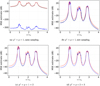Fig. 5 Quadratic error MSE estimates (dB scale). Black: reference; red: LOO; blue: PCe strategy.

4.2 PCe strategy: PC on error problem

Figure 5a presents the error estimate obtained by applying the PC methodology on equation (14) as a function of normalized pulsation, using the sampling points ${\underset{\_}{\xi }}_q$ as training data and the same polynomial order. This estimate is compared to the LOO estimate and the reference value.

The PC surrogate of the displacement, x_{P C}, is obtained as a linear combination of snapshots, each of them satisfying the linear equation (1). Thus the residue is equal to zero at this points, and finally we can conclude that the error computed using equation (18) at the sampling points ${\underset{\_}{\xi }}_q$ is nearly equal to zero (cf. Fig. 5b). Thus the sampling points of the error ${\underset{\_}{\xi }}_q$ should be different from the sampling points used for building the main surrogate.

Figures 5b to 5d present the mean square error at each frequency in dB scale, computed with the Monte Carlo reference technique (10⁵ samples), and with several orders for PC expansion: p^e = p (different points), p^e = p + 1 and p^e = p + 2.

It can be observed that the mean square error is well estimated, in particular for p^e > p, even if it leads to a higher numerical cost. Furthermore, the PC expansion suffers from the same drawbacks as stated previously: while the prediction remains accurate far from the resonance frequencies, the estimation of the error becomes less precise in the vicinity of resonance peaks. This is typically where the error is substantial, so this method cannot be deemed sufficiently accurate.

In the next subsection, we apply MbPCe expansion on the error problem.

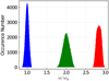Fig. 6 Empirical distributions of eigenvalues (105 realizations).

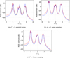Fig. 7 Quadratic error MSE estimates (dB scale). Black: reference; red: LOO; blue: MbPCe strategy.

4.3 MbPCe: modal basis PC expansion of the error problem

This part is dedicated to the case where the initial meta-model is obtained with a 1st-order PC approach, but the error surrogate is obtained using a MbPCe approach. The residual of the displacement surrogate acts as a source term, and the error can be estimated analytically as a linear combination of eigenmodes.

First, we present on Figure 6 the localization of the eigenvalues of the system (empirical histogram on the 10⁵ reference samples), and in Table 1 the mean and standard deviation of the eigenvectors.

Figure 7 presents the mean square error estimated for different levels of approximation of random eigenvectors.

A zero-order approximation of the eigenmodes at the nominal design yields results that are already fairly close to the reference value. The error on the MSE have the same order of magnitude as for the LOO estimate, and is even better far from eigenfrequencies. Around eigenfrequencies though, the error is badly estimated. However, using a first order surrogate of the eigenmodes leads to a very close agreement between the estimated MSE and the reference, using the same sampling points or not. This result is interesting because it means that, on the contrary of what has been observed in the previous section, no additional points are needed for the construction of the PC^e surrogate.

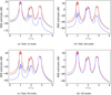Fig. 8 Quadratic error MSE estimates (dB scale). Black: reference; red: LOO; blue: OR-MbPCe strategy (full MbPCe in Figure 8d).

4.4 OR-MbPCe: one-mode reduction of modal basis PC expansion of the error problem

Figures 8a–8c present respectively the mean square error of the first component of ${\underset{\_}{e}}_{OR-MbPC}^{\left(1\right)}$, ${\underset{\_}{e}}_{OR-MbPC}^{\left(2\right)}$ and ${\underset{\_}{e}}_{OR-MbPC}^{\left(3\right)}$, when only one mode is included in the modal superposition. Figure 8d is the result of MbPC approach with all the modes.

The modes are approximated with a first-order PC expansion.

In these figures, the whole spectrum is plotted to illustrate the fact that the results are close to the reference only in the vicinity of the selected eigenfrequency. However, in an industrial context, one could of course compute the error level at the nominal eigenfrequency only, without drawing the whole spectrum.

5 Conclusion

In this paper, an innovative approach for assessing the approximation error introduced by a surface response method, specifically the polynomial chaos method, has been presented. Classic tools are based on the measure of the error on the training data set, or on a test data set, in order to approximate the global mean square error. On the contrary, the originality of this works lies in the resolution of a stochastic residual-based problem, enabling the derivation of a local approximation of the error. This additional problem is solved using a polynomial chaos expansion with additional parameters. It is shown that if both PC metamodels, displacement and error, are generated with the same approaches, sampling and parameters, the error value is equal to zero. Thus, an accurate error estimate can only be obtained by using a polynomial order for error approximation higher than the polynomial order for displacement approximation. Furthermore, a modal based strategy of the error problem has been tested with success, a first order approximation of the eigenmodes is often enough to estimate the error, and it is possible to use only one mode to estimate the error at the resonance peaks to reduce the numerical cost. This paper represents an initial effort to demonstrate the viability of this approach. Subsequent steps will focus on addressing more practical industrial scenarios, and we will delve into the pertinent technical specifics in upcoming publications.

Funding

The Article Processing Charges for this article are taken in charge by the French Association of Mechanics (AFM).

Appendix A Variables

References

All Tables

All Figures

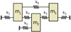	Fig. 1 3-dof system considered in the study, issued from [31].
In the text

	Fig. 2 Mean and 95%-confidence interval envelope of the displacement x1 and of the residual R1 on reference (105) points for a 1st-order PC approximation. Black line and grey envelope: reference results.
In the text

	Fig. 3 Mean and 95%-confidence interval envelop of the displacement x1 and of the residual R1 on reference (105 ) points for a 4th-order PC approximation. Black line and grey envelope: reference results.
In the text

	Fig. 4 MSE estimates for a 1st-order PC surrogate (plot in dB). Black: reference; blue: MSEtrain; red: LOO.
In the text

	Fig. 5 Quadratic error MSE estimates (dB scale). Black: reference; red: LOO; blue: PCe strategy.
In the text

	Fig. 6 Empirical distributions of eigenvalues (105 realizations).
In the text

	Fig. 7 Quadratic error MSE estimates (dB scale). Black: reference; red: LOO; blue: MbPCe strategy.
In the text

	Fig. 8 Quadratic error MSE estimates (dB scale). Black: reference; red: LOO; blue: OR-MbPCe strategy (full MbPCe in Figure 8d).
In the text

References

- A. Asadpoure, M. Tootkaboni, J.K. Guest, Robust topology optimization of structures with uncertainties in stiffness – application to truss structures, Comput. Struct. 89, 1131–1141 (2011) [CrossRef] [Google Scholar]
- M. Tootkaboni, A. Asadpoure, J.K. Guest, Topology optimization of continuum structures under uncertainty – a polynomial chaos approach,. Comput. Methods Appl. Mech. Eng. 201–204, 263–275 (2012) [CrossRef] [Google Scholar]
- G. Stefanou, The stochastic finite element method: Past, present and future, Comput. Methods Appl. Mech. Eng. 198, 1031–1051 (2009) [CrossRef] [Google Scholar]
- D. Xiu, Fast numerical methods for stochastic computations: a review, Commun. Comput. Phys. 5, 242–272 (2009) [Google Scholar]
- G. Fishman, Monte Carlo: Concepts, Algorithms, and Applications, Springer Science & Business Media (2013) [Google Scholar]
- R.E. Caflisch, Monte Carlo and quasi-Monte Carlo methods, Acta Numerica 7, 1–49 (1998) [CrossRef] [Google Scholar]
- R.G. Regis, C.A. Shoemaker, A stochastic radial basis function method for the global optimization of expensive functions, INFORMS J. Comput. 19, 497–509 (2007) [CrossRef] [MathSciNet] [Google Scholar]
- S. Volpi, M. Diez, N.J. Gaul, H. Song, U. Iemma, K.K. Choi, E.F. Campana, F. Stern, Development and validation of a dynamic metamodel based on stochastic radial basis functions and uncertainty quantification, Struct. Multidiscip. Optim. 51, 347–368 (2015) [CrossRef] [Google Scholar]
- J.P.C. Kleijnen, Regression and Kriging metamodels with their experimental designs in simulation: a review, Eur. J. Oper. Res. 256, 1–16 (2017) [CrossRef] [Google Scholar]
- H. Rostami, J.Y. Dantan, L. Homri, Review of data mining applications for quality assessment in manufacturing industry: Support vector machines, Int. J. Metrol. Qual. Eng. 6 (2015) [Google Scholar]
- E. Denimal, J.-J. Sinou, Advanced computational technique based on kriging and polynomial chaos expansion for structural stability of mechanical systems with uncertainties, J. Eng. Math. 130, 1–19 (2021) [CrossRef] [Google Scholar]
- M.A. El-Beltagy, A. Al-Juhani, A mixed spectral treatment for the stochastic models with random Parameters, J. Eng. Math. 132, 1–20 (2022) [CrossRef] [Google Scholar]
- N. Wiener, The homogeneous chaos, Am. J. Math. 60, 897–936 (1938) [CrossRef] [Google Scholar]
- R. Askey, J.A. Wilson, Some Basic Hypergeometric Orthogonal Polynomials that Generalize Jacobi Polynomials, Vol. 319. American Mathematical Soc., 1985 [Google Scholar]
- D. Xiu, George Em Karniadakis, Modeling uncertainty in steady state diffusion problems via generalized polynomial chaos, Comput. Methods Appl. Mech. Eng. 191, 4927–4948 (2002) [CrossRef] [Google Scholar]
- E. Jacquelin, S. Adhikari, J.J. Sinou, M.I. Friswell, Polynomial chaos expansion in structural dynamics: accelerating the convergence of the first two statistical moment sequences, J. Sound Vib. 356, 144–154 (2015) [CrossRef] [Google Scholar]
- E. Jacquelin, O. Dessombz, J.-J. Sinou, S. Adhikari, M.I. Friswell, Steady-state response of a random dynamical system described with padé approximants and random eigenmodes. Procedia Eng. 199, 1104–1109 (2017) [CrossRef] [Google Scholar]
- M.T. Reagan, H.N. Najm, R.G. Ghanem, O.M. Knio, Uncertainty quantification in reacting-flow simulations through non-intrusive spectral projection, Combust. Flame 132, 545–555 (2003) [CrossRef] [Google Scholar]
- R.A. Todor, C. Schwab, Convergence rates for sparse chaos approximations of elliptic problems with stochastic coefficients, IMA J. Numer. Anal. 27, 232–261 (2007) [CrossRef] [MathSciNet] [Google Scholar]
- X. Wan, G.E. Karniadakis, Long-term behavior of polynomial chaos in stochastic flow simulations, Comput. Methods Appl. Mech. Eng. 195, 5582–5596 (2006) [CrossRef] [Google Scholar]
- X. Wan, G.E. Karniadakis, An adaptive multi-element generalized polynomial chaos method for stochastic differential equations, J. Comput. Phys. 209, 617–642 (2005) [Google Scholar]
- B. Chouvion, E. Sarrouy, Development of error criteria for adaptive multi-element polynomial chaos approaches, Mech. Syst. Signal Process. 66, 201–222 (2016) [CrossRef] [Google Scholar]
- D.H. Mac, Z. Tang, S. Chénet, E. Creusé, Residual-based a posteriori error estimation for stochastic magnetostatic problems, J. Comput. Appl. Math. 289, 51–67 (2015) [CrossRef] [MathSciNet] [Google Scholar]
- G. Blatman, B. Sudret, An adaptive algorithm to build up sparse polynomial chaos expansions for stochastic finite element analysis, Prob. Eng. Mech. 25, 183–197 (2010) [CrossRef] [Google Scholar]
- G. Blatman, B. Sudret, Adaptive sparse polynomial chaos expansion based on least angle Regression, J. Comput. Phys. 230, 2345–2367 (2011) [CrossRef] [MathSciNet] [Google Scholar]
- C.V. Mai, B. Sudret, Hierarchical adaptive polynomial chaos expansions, in: UNCECOMP 2015 – 1st Int. Conf. Uncertain. Quantif. Comput. Sci. Eng., Vol. 229, May 2015, pp. 65–78, Crete, Greece, 2015 [Google Scholar]
- T. Duc Dao, Q. Serra, S. Berger, E. Florentin, Error estimation of polynomial chaos approximations in transient structural dynamics, Int. J. Comput. Methods 17, 2050003 (2020) [CrossRef] [MathSciNet] [Google Scholar]
- T. Butler, P. Constantine, T. Wildey, A posteriori error analysis of parameterized linear systems using spectral methods, SIAM J. Matrix Anal. Appl. 33, 195–209 (2012). [CrossRef] [MathSciNet] [Google Scholar]
- L. Mathelin, O. Le Maitre, Dual-based a posteriori error estimate for stochastic finite element Methods, Commun. Appl. Math. Comput. Sci. 2, 83–115 (2007) [CrossRef] [MathSciNet] [Google Scholar]
- K. Dammak, S. Koubaa, A. El Hami, L. Walha, M. Haddar, Numerical modelling of vibro-acoustic problem in presence of uncertainty: application to a vehicle cabin, Appl. Acoust. 144, 113–123 (2019) [CrossRef] [Google Scholar]
- M. Ghienne, C. Blanzé, L. Laurent, Stochastic model reduction for robust dynamical characterization of structures with random parameters, Comptes Rendus Méc. 345, 844–867 (2017) [Google Scholar]
- M. Berveiller, B. Sudret, M. Lemaire, Stochastic finite element: a non intrusive approach by regression, Eur. J. Comput. Mech. 15. 81–92 (2006) [CrossRef] [Google Scholar]
- G. Blatman, B. Sudret, Sparse polynomial chaos expansions and adaptive stochastic finite elements using a regression approach, Comptes Rendus Mec. 336, 518–523 (2008) [CrossRef] [Google Scholar]
- D.M. Allen, Mean square error of prediction as a criterion for selecting variables, Technometrics 13, 469–475 (1971) [CrossRef] [Google Scholar]
- A.M. Molinaro, R. Simon, R.M. Pfeiffer, Prediction error estimation: a comparison of resampling methods, Bioinformatics 21, 3301–3307 (2005) [CrossRef] [PubMed] [Google Scholar]
- M. Stone, Cross-validatory choice and assessment of statistical predictions, J. R. Stat. Soc. Ser. B 36, 111–147 (1974) [Google Scholar]
- B. Efron, R. Tibshirani, An Introduction to the Bootstrap, Chapman and Hall, New York, 1993 [Google Scholar]
Cite this article as: Q. Serra, E. Florentin, Verification of polynomial chaos surrogates in the framework of structural vibrations with uncertainties, Mechanics & Industry 24, 42 (2023)