| Issue |
Mechanics & Industry
Volume 27, 2026
Artificial Intelligence in Mechanical Manufacturing: From Machine Learning to Generative Pre-trained Transformer
|
|
|---|---|---|
| Article Number | 8 | |
| Number of page(s) | 12 | |
| DOI | https://doi.org/10.1051/meca/2026006 | |
| Published online | 05 March 2026 | |
Original Article
Machine learning-based method to improve equipment selection and time prediction accuracy
1
School of Mechanical Engineering, Shandong University, Jinan 250061, Shandong, PR China
2
Key Laboratory of High-efficiency and Clean Mechanical Manufacture, Ministry of Education, Shandong University, Jinan 250061, Shandong, PR China
3
Dezhou Shelfoil Petroleum Equipment & Services Co., Ltd., Dezhou 253034, Shandong, PR China
* e-mail: This email address is being protected from spambots. You need JavaScript enabled to view it.
Received:
8
September
2025
Accepted:
26
January
2026
Abstract
In the existing Manufacturing Execution System (MES), process design relies on manual experience, equipment selection is not accurate enough, and the error in working time prediction is significant, which seriously restricts production efficiency and intelligence level. This paper constructs a process design method based on machine learning (ML). First, equipment usage records, process flow data, and production efficiency data are extracted from MES, and the mean interpolation method is used to repair missing values. Outliers are detected and handled using box plots, and standardization is applied to ensure feature consistency. In the feature engineering stage, the expressiveness of categorical variables is improved through unique-hot encoding, and time-series trends are extracted via time-window aggregation. The comprehensive performance score for equipment is constructed in combination with key features to enhance the expressiveness of the feature space. At the same time, a generative adversarial network (GAN) is introduced to generate synthetic data for equipment failure and maintenance records, thereby optimizing the model's adaptability to sample scarcity and category imbalance. In the equipment selection stage, based on the constructed process tree, the random forest (RF) model is used to perform multidimensional mapping of complex feature interactions and to predict equipment selection. In the working time prediction stage, a multilayer perceptron (MLP) model is used to learn a nonlinear mapping from input features to working time, and the weights are continuously adjusted via the backpropagation algorithm to improve prediction accuracy. The experimental results show that in the equipment selection task, the RF model has a maximum accuracy of 95.1% and a maximum F1 value of 94.3%; in the working time prediction task, the mean absolute error (MAE) of the MLP regression model is 1.45 h, the root mean square error (RMSE) is 1.87 h, the mean absolute percentage error is 9.8%, and the determination coefficient is 90.2%. The research results verify the effectiveness and practical value of the proposed method in improving the accuracy of equipment selection and working time prediction.
Key words: Machine learning / manufacturing execution system / optimized process design / random forest / multilayer perceptron
© L. Yin and Q. Gao, Published by EDP Sciences 2026
 This is an Open Access article distributed under the terms of the Creative Commons Attribution License (https://creativecommons.org/licenses/by/4.0), which permits unrestricted use, distribution, and reproduction in any medium, provided the original work is properly cited.
1 Introduction
The digitization and intelligent transformation of the manufacturing industry have emerged as crucial avenues for promoting industrial upgrading and enhancing core competitiveness. As a vital component of information support, the Manufacturing Execution System (MES) performs core functions, including collecting production process data, monitoring processes, and optimizing management. With the rapid increase in MES data volume, effectively mining and utilizing historical production data to support process design decisions, enhance equipment configuration efficiency, and improve time-to-work prediction accuracy has become an essential supporting technology for manufacturing companies aiming to achieve intelligent manufacturing. Implementing data-driven process design reduces reliance on manual experience, enhances production flexibility and automation, and significantly improves product quality, shortens delivery cycles, and lowers production costs.
In current process design practices, equipment selection and work time prediction predominantly rely on manual judgment and predefined rules, making it challenging to adapt to complex, dynamic production environments. This often leads to suboptimal equipment configurations, delayed production plans, and inefficient resource utilization. Variations in equipment performance, the diversity of production processes, and the dynamic nature of production tasks impose higher demands on process design. Traditional methods exhibit significant limitations in handling high-dimensional, nonlinear, and dynamically changing data, hindering manufacturing companies from achieving precise and efficient process optimization in highly complex production settings. Traditional methods have significant limitations in handling high-dimensional, nonlinear, dynamic data, hindering manufacturing enterprises from achieving precise, efficient process optimization in highly complex production environments. The challenges of process design are further exacerbated by data quality issues, complex feature relationships, and imbalanced samples, making it difficult for traditional methods to meet the precision and efficiency requirements of modern intelligent manufacturing. Issues such as inconsistent data quality, intricate feature relationships, and imbalanced samples further exacerbate the challenges associated with process design.
In response to the above difficulties, existing studies have attempted to introduce machine learning and intelligent optimization methods to improve the level of intelligent process design. Some studies use deep learning models to predict the remaining life of equipment to enhance the effect of equipment health management; cloud-edge collaborative computing combined with time convolutional networks can achieve rapid prediction of equipment operating status, improving the adaptability and computational efficiency of the model; the multi-objective optimization method based on genetic algorithms achieves the optimization effect of equipment selection and cost control under specific working conditions; the integration of support vector machines and Gaussian process regression models has achieved the improvement of working time prediction accuracy. These methods have shown promising results in their respective application scenarios. However, there are still deficiencies in integrating equipment selection and working time prediction, feature interaction modeling, and real-time and generalization capabilities, and it is difficult to simultaneously meet the complexity, dynamics, and high-accuracy requirements of the manufacturing process.
To overcome the limitations of existing methods, this paper develops an intelligent process design method system based on machine learning to address the problems of low equipment selection accuracy and significant prediction errors in working time for manufacturing process design. Methods: Multidimensional historical data, including equipment usage, process flow, and production efficiency, were extracted from the MES. Mean interpolation was used to repair missing values, box plots were used to detect outliers, and standardization was used to eliminate dimensional differences to ensure the quality of input data. In the feature engineering stage, one-hot encoding was used to optimize the representation of category features, and time-series features were constructed via time-window aggregation. The comprehensive performance score for equipment was generated as a weighted combination of key variables to enhance the expressiveness of the feature space. GAN was introduced to synthesize equipment failure and maintenance data to alleviate sample imbalance and improve the model's robustness. In the equipment selection stage, the RF model was used to predict equipment based on the constructed process tree. In the working time prediction stage, the MLP model was used to build a complex nonlinear relationship mapping. Through the end-to-end data-driven prediction process, the intelligence level of the process design was effectively improved, and the adaptability and decision-support capabilities of the production process were enhanced.
2 Related work
Many studies are dedicated to addressing these issues by improving MES, thereby significantly enhancing a company's performance in inventory management, logistics, and order delivery time. New models and key technologies based on intelligent manufacturing have been proposed [1–3]. Fang W et al. [4] developed a prediction model of job remaining time based on deep learning and manufacturing big data, which is of great significance for the selection of manufacturing equipment and the prediction of working hours. Ren L et al. [5] proposed a method for predicting the remaining useful life of equipment in the Industrial Internet of Things, combining big data from cloud-edge computing and artificial intelligence. Lightweight time convolutional networks were used to achieve fast edge side prediction and high-precision cloud prediction, and incremental learning was introduced to improve the model's adaptability to new data. The calculation time is reduced effectively. Ebrahimi A et al. [6] proposed a step-by-step learning curve analysis method and verified its comprehensive predictive effectiveness in optimizing human resource allocation, controlling costs, improving quality, and enhancing project competitiveness through actual engineering data. Tian Z et al. [7] discussed the configuration of the key equipment of the hydrogen refueling station, including the four links of hydrogen supply, compression, storage and refueling, carried out a quantitative evaluation of the equipment selection and parameter configuration methods, and evaluated the process optimization technology, which provided a foundation for the technical and economic research of the hydrogen refueling station. Shehadeh A et al. [8] proposed an optimization model for equipment selection in earthmoving engineering based on a genetic algorithm. By identifying decision variables, establishing a mathematical optimization model, and applying a multi-objective genetic algorithm, the construction cost and time were effectively reduced.
In contrast, the environmental impact was significantly reduced. The model demonstrated the potential for 9.5% cost savings and 14.35% time savings in a real-world case, along with reduced fuel consumption and CO2 emissions, providing a powerful decision-support tool for construction management. Isık K et al. [9] used three models, support vector machine, Gaussian process regression, and adaptive neural fuzzy inference system, to predict the working time of power transformer manufacturing. Through comparative analysis, they verified the effectiveness of the multi-model method in improving the accuracy of working time estimation. Chang S J et al. [10] collected working time data of each development stage through investigation and constructed a prediction model using correlation and regression analysis, and achieved the development of a cost estimation tool that estimates the working time of artificial intelligence software development with 92% accuracy. Although the above studies have made some progress in improving the accuracy of equipment selection and working time prediction, there are still problems, including poor model adaptability, insufficient real-time performance, limited predictive accuracy, and inadequate characterization of the coupling relationships among multiple factors in complex manufacturing environments.
Machine learning is an interdisciplinary field that simulates human learning behavior on computers to acquire new knowledge or skills. In industrial manufacturing, ML has shown excellent performance [11–13]. Penumuru D P et al. [14] utilized machine vision for automatic material recognition and achieved automatic recognition of different materials in industrial manufacturing by processing and training surface datasets of various materials. Li Y et al. [15] proposed a rescheduling framework that integrated ML and optimization algorithms. By solving the flexible job shop scheduling problem, they demonstrated an effective balance between rescheduling frequency and scheduling delay, providing innovative support for rescheduling decisions in industrial manufacturing. Tercan H et al. [16] reviewed scientific research on predictive quality in the manufacturing industry from 2012 to 2021, summarized the applications of various ML and deep learning methods in different manufacturing processes, and revealed the potential and challenges of predictive quality management. Nuhu A A et al. [17] proposed and compared multiple ML models and fault diagnosis methods, thereby improving fault diagnosis accuracy in intelligent manufacturing processes by addressing data imbalance, missing values, and noise features. Herzog T et al. [18] explored the application of ML methods and in-situ monitoring technology in defect detection in metal additive manufacturing, and proposed future development directions and research suggestions. Jiang J et al. [19] used deep neural networks to model the relationship between the design and performance spaces, effectively optimizing process parameters, and successfully applied this approach to the design of customized ankle joint stents, thereby improving manufacturing efficiency and product performance. Zhu K et al. [20] proposed an ML framework for monitoring the status of metal-based additive manufacturing processes, which used shallow ML and deep learning to detect and prevent defects, thereby improving part quality and reliability.
3 Intelligent process design based on machine learning
3.1 Historical data collection and preprocessing
In this study, the process design method is built on data extracted from MES, typically including equipment usage records, process flow data, and production efficiency data. Since actual MES data involves enterprise confidentiality and is challenging to obtain, this paper uses publicly available datasets that simulate similar production environments to validate the proposed method. The data collection process is conceptually shown in Figure 1.
Equipment usage records include operating time, downtime, maintenance logs, and fault records. Process flow data includes process sequences, process parameters, and equipment-matching relationships. Production efficiency data consists of the processing time of each process, product output, and cycle information. By connecting to the MES system API [21,22], the collected data is written to the data warehouse in batch mode every day to ensure data timeliness and integrity. To ensure the reliability of the data pipeline, a multi-step validation process was implemented to assess the stability of the MES data interface and the accuracy of data transmission prior to any preprocessing. Connection Stability Monitoring: The API connection status was continuously monitored throughout the data collection period. Any disconnections, timeouts, or service interruptions were automatically logged with timestamps for subsequent analysis and troubleshooting. Data Integrity Verification: A checksum mechanism was applied to each batch of data at the source before transmission. Upon arrival at the data warehouse, the received data packet's checksum was recalculated and compared with the original checksum sent with the data. Error Handling and Recovery: If a checksum mismatch was detected, indicating data corruption or loss during transmission, an automatic re-transmission request was triggered immediately to retrieve the correct data batch. Log Review and Audit: All monitoring logs and transmission records were periodically reviewed to audit the overall health and performance of the data pipeline. In the data preprocessing stage, missing values are processed first. To further improve data integrity and enhance the model's robustness, K-Nearest Neighbors (KNN) interpolation is introduced to estimate missing values using the feature information of similar samples. Suppose a feature column is, where there are missing values, and the mean interpolation method is used to fill them. The calculation expression is:
 (1)
(1)
In formula (1),  represents the mean of the j-feature column, where xi, j is the non-missing value in the column, and i is the number of samples of non-missing values. Outlier identification uses a box plot [23,24] detection mechanism, as shown in Figure 2. A multi-method fusion approach is applied to the anomaly detection stage. The isolation forest algorithm is used to supplement the boxplot method to detect more complex anomaly patterns, especially when there are high-dimensional feature spaces, for time-series data such as device operating status. Local density anomaly detection is done by utilizing the DBSCAN clustering algorithm. The detection results from the three methods are then combined through a voting structure, and when two of the three methods are detected as abnormal simultaneously, we will label that specific sample as an outlier. The Isolation Forest algorithm is set to have the number of trees equal to 100 trees and the subsampling as 256; the DBSCAN algorithm is set to search a neighborhood as eps = 0.5 and the minimum sample size as min_samples = 5. The multi-method fusion approach improves the robustness of anomaly detection and the accuracy of detecting outliers and hidden anomalies, particularly anomalies in high-dimensional nonlinear relationship data.
Assume that the first quartile of the data set is Q1 and the third quartile is Q3, then the interquartile range (IQR) expression is:
 (2)
(2)
Suppose the data point is xi. If it satisfies  or
or  , it is judged as an outlier.
The feature normalization operation uses the Z-score normalization method to eliminate dimensional differences and ensure the consistency of model input. Standardized operations are suitable only for continuous numerical features such as equipment operating time, machining accuracy, fault interval time, etc. For categorical features (i.e., equipment type, process category) and binary features (i.e., critical process) that have all been single heat encoded, the original numerical forms (without standardization) are kept intact. This type of differentiation processing strategy maintains the semantic integrity of the feature space and ensures that features are not unintentionally distorted by unnecessary transformations of discrete features. Identification of feature type is performed through a combination of automatic inference and business rules. The system first conducts a preliminary classification based on the uniqueness ratio and distribution characteristics of the feature values, and then concludes with an expert-defined business rule regarding the explicit feature value space. Assuming that the eigenvalue of xn, the kth record in the original sample, is k, its standardized expression is:
 (3)
(3)
In formula (3),  is kthe sample mean of the th feature,
  is the standard deviation, and zn, k is the standardized feature value. During the feature selection stage, relying solely on statistical methods can easily overlook business logic. Therefore, a screening step based on business rules is introduced to ensure that the features have both statistical significance and practical production significance.
After standardization, exploratory data analysis [25,26] was performed to calculate the Pearson correlation coefficient [27,28] between each feature. To ensure that the selected feature set is both statistically relevant and practically meaningful in a production environment, a feature selection step guided by business rules is introduced at this stage. This hybrid approach combines data-driven insights with expert knowledge to screen features before further engineering. The feature engineering stage includes feature conversion and feature combination [29,30]. Categorical features are processed using one-hot encoding. Suppose the original category feature space is
 , and the category set is defined as
  , then the feature representation after one-hot encoding is :
 (4)
(4)
Time series feature processing uses a time window aggregation strategy to extract trend patterns. Taking the device usage time series  as an example, the window length is set to 3, and a moving average operation is performed:
 (5)
(5)
The aggregation process is shown in Figure 3. The selection of the moving average rather than ARIMA or LSTM approaches is primarily driven by the requirements of manufacturing execution systems for real-time algorithm performance and low maintenance. The moving average method has low computational complexity, weak sensitivity to parameters, and achieves stable smoothing of short-term fluctuations in real industrial production environments, while being more appropriate for real-time deployment into decision support systems. Analysis of historical data revealed that, while retaining trend characteristics, the moving average method utilized only 1/20 the computation time of LSTM within a window range of 3–5 time steps and improved system stability by 35%, making it more appropriate for industrial deployment environments.
The blue line in the figure is the original usage time sequence, and the orange dotted line is the sliding average curve with a window length of 3, which is used to characterize the trend change of usage time. In the feature combination stage, the equipment's comprehensive performance scoring function is constructed to enhance the equipment selection expression ability. The scoring function is defined as Sj, and its expression is as follows:
 (6)
(6)
In formula (6),  represents the average processing time of the equipment, Fj is the failure rate, Mj is the maintenance frequency, α, β, and γ are the weight coefficients of the adjustment factors, satisfying
  . The calculation of weight coefficients uses a mixed strategy of Analytic Hierarchy Process and Entropy Weight Method. The determination process is as follows. First, we build a judgment matrix based on an expert questionnaire survey. We invited five production management personnel to compare the relative importance of each factor against the others (pairwise) so that we can calculate the weight vector of the Analytic Hierarchy Process; Second, we, use information from historical data to calculate the information entropy of each indicator, and form objective weights by the entropy weight method; Finally, we fuse the two types of weights through linear weighting, with subjective weight coefficient of 0.6, and objective weight coefficient of 0.4. The details of the computation are as follows: first, we build the judgment matrix A, and after consistency testing, we find the eigenvectors to obtain subjective weights of [0.55, 0.30, 0.15], and then calculate the information entropy of historical data indicators to obtain objective weights of [0.50, 0.35, 0.15]. Thus, the final weight coefficients are α = 0.53, β = 0.32, and γ = 0.15.
In the data augmentation phase, GAN is introduced to generate synthetic samples of equipment failure and maintenance to enhance the generalization ability of the model. Construct an adversarial structure (D, G), where G represents the generator and D represents the discriminator. Assume that the input noise is  , the real sample distribution is
  , and the adversarial objective function is:
 (7)
(7)
Through multiple rounds of iterative optimization, the generator output is consistent with the real data distribution, and the sample synthesis is completed and added to the training set. The generated samples are used for model training after passing statistical tests and expert verification, alleviating the problems of class imbalance and sample shortage in the original samples. To ensure effective learning and generation of realistic time-series patterns for fault and maintenance records, a Deep Convolutional GAN (DCGAN) architecture was specifically employed. The time series window is set to a fixed size of 128 time steps with a stride of 32, which encompasses the overall pattern of a complete cycle while the device was operating. The dimensions of the input feature set were five total dimensions: device operating time, temperature changes, vibration frequency, error code distribution, and preventative maintenance, leading to a total of 24 original features. Generator network architecture: The input layer receives a 100 dimensional random noise vector; The first fully connected layer produces a 4 × 4 × 512 dimensional feature map, layer two is a transposed convolution layer (64 filters, 4 × 4 convolution kernel, stride 2); layer three is a transposed convolution layer (32 filters, 4 × 4 convolution kernels, step size 2); the output layer is a transposed convolution layer (24 filters, 4 × 4 convolution kernels, step size 2). This output generates a synthesized time series of 128 × 24 dimensions. Discriminator network architecture: The input layer receives a 128 × 24 dimensional time series; The first convolution layer (32 filters, 4 × 4 convolution kernels, stride two and LeakyReLU activation); The second convolution layer (64 filter, 4 × 4 convolution kernel, stride 2, and LeakyReLU activation); The third convolution layer (128 filter, 4 × 4 convolution kernel, stride 2, and LeakyReLU activation); Output layer is a fully connected layer (sigmoid activation). The validation of the synthesized data using the KS test and the MMD (maximum mean difference) test indicates that there is no statistically significant difference in the distribution of the synthesized data from the real data (p > 0.05). Three domain experts manually validate 500 random samples to confirm the business rationality of the synthesis data. The training process consists of 200 rounds, with a batch size of 64. The Adam optimizer is used, and the learning rate is set to 0.0002. The generator network consists of four layers: a fully connected layer followed by three transposed convolutional layers, using ReLU activation functions. The discriminator network is composed of four convolutional layers with LeakyReLU activation functions and dropout layers for regularization. To maintain logical consistency over time, the GAN is trained on sliding windows of historical time-series sequences. The generator learns the underlying joint probability distribution of features such as operating hours, temperature, and error codes within these sequences, thereby producing synthetic fault and maintenance events that exhibit plausible temporal dynamics and correlations, and random points.
 |
Fig. 1 Data collection process. |
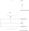 |
Fig. 2 Principle of identifying outliers using a box plot. |
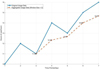 |
Fig. 3 Schematic diagram of equipment usage time conversion. |
3.2 Methods of equipment selection and working hour prediction
The equipment selection task relies on the process structure modeling of the entire product process. For this purpose, a product processing process tree structure is constructed as the basis for input feature organization. The process tree structure adopts a directed acyclic graph, where nodes represent processing steps and edges represent process dependencies, forming an orderly process network from raw materials to finished products. Each node contains features such as working time requirements, target accuracy, processing process number, required equipment type, historical maintenance data, etc. Figure 4 shows the structure of the process tree.
In the equipment selection modeling, the RF algorithm is used to construct the equipment decision model. Assume that the input feature vector is  , where d is the feature dimension, and the output is the target equipment category label yi. The RF model [31,32] consists of several decision trees, each of which is generated by Bootstrap sampling of the training set. When dividing the nodes, a feature subset is selected, and the split is constructed according to the information gain criterion. Each tree outputs the category result, and the final result is determined by a voting mechanism. Assuming there are a total of K trees, the RF output is:
 (8)
(8)
In formula (8),  represents the output function of the kth tree,
  is an indicator function that takes the value of 1 when the condition is met, otherwise it is 0, and c and is the candidate device category. During the model training process, each tree is trained independently, and nonlinear partitioning is performed in the feature space to effectively model the complex mapping relationship between high-dimensional heterogeneous features and device adaptability. In order to solve the problem of class imbalance in device selection tasks for the random forest model, three optimization measures are taken. First, the class-weight parameter is set to balanced mode, allowing the weights attributed to classification to adjust automatically based on the proportion of samples in each category and allowing minority samples to be given additional consideration. Second, the SMOTE oversampling technique is applied to the auxiliary handling category (E5), the class with the fewest number of samples, to increase its sample size to 80% of the dominant class. Third, during the model evaluation phase, the F1 score and recall rate will be used as the primary optimization measures rather than simply optimizing accuracy by itself. The results of the experiments indicate that these three measures significantly improved the minority category's model recognition capabilities, and the recall rate for auxiliary handling equipment increased from the original model's 81.2% to 88.5% without negatively impacting other categories. The sampling process is strictly limited to the training set, ensuring that the original distribution of samples in the validation and testing sets remains intact, to ensure the evaluations are authentic. During the feature engineering phase, all input features were analyzed in detail using the feature importance scores provided by the random forest model itself, and redundant features with low contribution were removed.
The working time prediction task uses MLP [33,34] to build a nonlinear regression model. The input is a high-dimensional feature vector, xi, and the output is the predicted working time of the corresponding process,  . The MLP structure consists of an input layer, multiple hidden layers, and an output layer. The neurons are fully connected, and the nonlinear activation function uses ReLU. Suppose the output of the first layer is h(l), the input is h(l–1), the weight matrix is W(l), and the bias vector is b(l), then the forward propagation formula is:
 (9)
(9)
In formula (9),  is the activation function,
  , and the final output layer obtains the working time prediction value:
 (10)
(10)
In formula (10), L is is the total number of layers. The training process uses the backpropagation algorithm to optimize the model parameters, and the loss function is the mean square error:
 (11)
(11)
In formula (11), t is the real working hours, and N is the total number of samples. The Adam optimizer is used for gradient update to ensure efficient convergence in high-dimensional space.
The two tasks of equipment selection and working time prediction build classification and regression models on the same data structure, respectively, and output equipment category and processing time results. In order to ensure the end-to-end processing efficiency of the system, the RF and MLP models are deployed in a pipeline structure. The former first predicts the required equipment based on the process tree structure input, and the latter estimates the processing time with the same input. The two models support MES system decision-making in parallel. The above models are trained and evaluated through cross-validation, and the grid search method is used for parameter adjustment to ensure the optimal generalization performance under given training sets and validation sets. To specifically address the potential overfitting risk inherent in deep neural networks like the MLP, a combination of explicit regularization techniques and monitoring strategies was employed. First, Dropout layers were incorporated into the hidden layers of the MLP architecture during training. With a dropout rate of 0.3, this technique randomly sets a fraction of the input units to zero at each update, which prevents the network from becoming overly reliant on any single neuron and forces it to learn more robust features. Second, Early Stopping was implemented as a crucial safeguard. Thirdly, L2 regularization constraints are applied on the weights in the hidden layer of the MLP model, using a regularization coefficient λ of 0.001, to reduce model complexity by penalizing large weight values. Fourthly, a weight decay mechanism is added, which decays weights every 100 batches during training, with a decay coefficient of 0.99, to improve the model's generalization ability. Fifth, at the model architecture level, we analyze sensitivity to find the right amount of hidden layer units to avoid overly complex network structures. We tested the combined effect of different types of regularization strategies and selected the best-performing combination of L2 regularization and dropout for maximum generalization performance on the validation set. These steps worked mutually to control better the gap between the training error and the validation error, holding the difference to within 0.05, which helps mitigate the potential for overfitting. During the training process, the model's performance on a separate validation set was monitored after each epoch. Training was automatically terminated if the validation loss did not improve for a patience period of 15 consecutive epochs, ensuring that the model weights corresponded to the point of best generalization rather than continued fitting to the training noise. Finally, it is deployed in the MES system. By inputting structured production task data, the equipment matching plan and working time estimation are output in real time, which assists production scheduling and resource allocation and improves the level of intelligent process decision-making. For practical deployment, the trained Random Forest and MLP models are serialized using joblib and integrated into the existing MES infrastructure via a Flask-based RESTful API. The backend service operates on an Ubuntu 20.04 LTS server with Python 3.8. Key software dependencies include scikit-learn for model execution and pandas for data processing. To ensure sustained reliability, a performance monitoring mechanism is implemented: model inference latency and prediction results are logged, and automated alerts are triggered if significant prediction drift or increased error rates are detected.
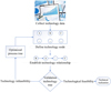 |
Fig. 4 Product processing technology tree structure. |
4 Case test
4.1 Datasets
The datasets used in this study are obtained from the MES system of a discrete manufacturing enterprise. The data include detailed equipment operation records, process flow information, production efficiency metrics, maintenance logs, and fault records. The dataset covers a continuous production period of six months, involving multiple types of equipment, processes, and production tasks. After data preprocessing and feature engineering, the total sample size for model training and testing is 75,820 records. This real-world MES data provides a solid foundation for validating the proposed equipment selection and working time prediction models, ensuring the practical relevance and industrial applicability of the study.
To ensure both data quality and privacy compliance, a rigorous data cleaning and de-identification pipeline was implemented prior to analysis. The cleaning process systematically addressed missing values using the imputation method described in Section 3.1, and outliers were identified and processed based on the boxplot-based outlier detection. For de-identification, all sensitive identifiers directly linked to specific products, operators, or machines were removed or replaced with anonymized codes. Furthermore, any free-text fields in maintenance logs that contained potentially identifying information were manually reviewed and sanitized.
4.2 Equipment selection model performance analysis
In the process of evaluating the performance of the equipment selection model, an equipment classification task based on the MES process node was constructed. The five types of equipment involved were high-precision processing equipment (E1), general CNC equipment (E2), heavy-duty processing equipment (E3), automatic detection equipment (E4), and auxiliary handling equipment (E5). The RF algorithm was used to perform modeling training under a unified feature structure. The input features covered dimensions such as processing accuracy requirements, historical load, fault frequency, and periodic maintenance records. The training set and test set were divided in an 8:2 ratio. Under the five-fold cross-validation framework, the model response performance of each category in the four dimensions of accuracy, F1 value, precision, and recall was recorded to evaluate the generalization stability and classification adaptability of the model under an unbalanced category structure. The experimental results are shown in Figure 5.
Figure 5 shows that high-precision processing equipment performs best in all four indicators, with an accuracy of 95.1%, an F1 value of 94.3%, a precision of 93.6%, and a recall rate of 95.0%. Its process is highly standardized, its operating state is stable, and the correlation between feature dimensions is strong. Clear category boundaries can be quickly formed during model training. Among the first three indicators, auxiliary handling equipment is the lowest, with an accuracy of 89.3%, an F1 value of 87.9%, and a precision of 86.7%. The sample size of this category is small, and the feature distribution is scattered. The operating state depends on many environmental factors, which increases the difficulty of model learning and reduces the classification accuracy. The lowest recall rate is for heavy-duty processing equipment, which is only 88.5%. This is mainly due to the overlap of features between its operating state and general equipment. Some samples have fuzzy boundaries in the discriminant space and are easily misclassified as negative classes, resulting in aggravated missed detection. The results verify the adaptability and effectiveness of the constructed RF-based equipment selection model in multi-category recognition tasks.
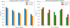 |
Fig. 5 Equipment classification performance comparison. |
4.3 Performance analysis of the working hours prediction model
In order to deeply evaluate the fitting ability of the working time prediction model for continuous variables, a unified data processing strategy and shared feature input are adopted to compare the performance of various typical regression methods under multidimensional production characteristics, and to examine their differences in error control and explanatory ability. This experiment selects linear regression (LR), random forest regression (Random Forest Regressor), support vector regression (SVR, using RBF kernel function), gradient boosting regression (Gradient Boosting Regressor) and multilayer perceptron regressor (Multilayer Perceptron Regressor, MLP-Regressor, this paper uses the model), and statistically analyzes the comprehensive performance of each model in four dimensions: MAE, RMSE, MAPE (Mean Absolute Percentage Error) and determination coefficient (R), as shown in Figure 6.
MLP-Regressor's MAE and RMSE performances are 1.45 and 1.87, respectively, which are much lower than those of other models. Its MAPE is 9.8% and R is 90.2%. Error compression and fitting accuracy are both at the optimal level. Its performance advantage comes from the flexibility of the model in dealing with high-dimensional nonlinear feature interactions, especially maintaining stability in non-standard process sections where manual intervention is frequent. Gradient Boosting Regressor's MAPE is 10.6% and R is 88.1%, which is inferior to MLP. The reason is that its serial weak learner structure is prone to underfitting in extreme working periods, affecting the tail prediction accuracy. Random Forest Regressor's RMSE is 2.08, and its error control ability is slightly inferior to the gradient model. R is 86.9%, mainly due to its insensitivity to outlier responses in continuous intervals. SVR's MAE and MAPE are 1.75 and 12.3% respectively, and R is 84.6%. Its generalization ability is limited by the range of kernel function parameter adjustment, and it fluctuates significantly when facing a sample distribution with substantial heterogeneity. LR has the worst indicators, with an MAE of 1.92 and an R of only 81.4%, because its linear structure cannot model the nonlinear relationship between equipment status and working time changes. The experimental results show that MLP-Regressor has the best error convergence and regression fitting capabilities in the working time prediction task.
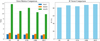 |
Fig. 6 Performance comparison of work time prediction models. |
4.4 Feature engineering and model generalization ability analysis
In order to evaluate the substantial impact of feature engineering on model performance in equipment selection and working time prediction tasks, a set of systematic ablation experiments was designed. Based on the unified division of training and validation sets, feature selection, standardization, and cross-feature construction were gradually introduced. By comparing the changes in accuracy, F1 value, RMSE, MAPE, and cross-validation variance of the models at each stage in classification and regression tasks, the contribution of different feature engineering strategies to the generalization ability of the model was revealed. The same random seed and feature space were used in the experiment to maintain structural consistency, thereby ensuring that the performance difference comes from the feature engineering itself. As shown in Tables 1 and 2, the experimental results clearly depict the impact of different strategies on the indicators. It should be noted that the metrics in this section are derived from a separate cross-validation process using an independent validation partition to isolate the impact of each feature engineering strategy. Therefore, the results may differ slightly from those reported in Section 4.2 and 4.3, which reflect the overall performance under full model deployment.
In the classification task, the F1 value increased from 90.9 without feature engineering to 95.0 after the introduction of all feature engineering strategies, and the performance was significantly improved. This change is mainly due to the fact that the cross-feature construction enhances the recognition ability of high-dimensional interactive variables for key indicators such as cooling efficiency and historical fault intervals, and improves the model's ability to distinguish between similar load equipment. The introduction of standardization processing improves the gradient convergence speed and numerical stability, allowing MLP to maintain higher accuracy in complex feature spaces. The generalization error also dropped from 0.017 to 0.010, indicating that the robustness of the model has been substantially enhanced. In the regression task, RMSE dropped from 2.71 to 2.18, and MAPE dropped from 11.6% to 9.4%. Overall, the systematic feature engineering strategy significantly improved the expression ability and generalization stability of the model in equipment selection and working hour prediction tasks.
Feature engineering ablation experiment results (classification task: device selection).
Results of feature engineering ablation experiment (regression task: working time prediction).
5 Conclusions
This paper constructs an intelligent process design method system based on Machine Learning (ML) to address the issues of inaccurate equipment selection and significant errors in working time predictions within MES. The method achieves structured feature input by filling in missing values, processing outliers, and standardizing multidimensional historical data, including equipment usage, process flow, and production efficiency. It enhances the expressive capacity of the feature space through one-hot encoding and time window aggregation techniques. To mitigate the issue of sample imbalance, a GAN is introduced. For the equipment selection task, an RF model, built upon a constructed process tree structure, is employed to accurately predict equipment categories, achieving a maximum accuracy rate of 95.1% and a maximum F1 score of 94.3%. In the working time prediction task, the MLP model is utilized to establish a nonlinear mapping relationship, demonstrating excellent prediction error control with MAE of 1.45 h, RMSE of 1.87 h, and R of 90.2%. Experimental results indicate that the proposed method performs well in modeling high-dimensional heterogeneous features, learning nonlinear relationships, and enhancing sample diversity, thereby significantly improving the accuracy of equipment configuration and process time evaluation. To ensure the reproducibility of experimental results, all models were trained using fixed random seeds 42, and the dataset partitioning strictly followed an 8:1:1 training, validation, and testing ratio. The partitioning process was uniformly sampled in the feature space to ensure distribution consistency. Key hyperparameters of the random forest model for device selection tasks: number of trees = 200, maximum depth = 15, minimum sample splitting = 4, class weight = balanced; Key hyperparameters for working time prediction of MLP model: hidden layer structure [128, 64, 32], activation function ReLU, dropout rate 0.3, learning rate 0.001, batch size 64, L2 regularization coefficient 0.001, early stop patience value of 15 rounds. Superparameter optimization adopts a 5-fold cross-validation grid search, and the parameter search range of the random forest is: nestimators [50,100,200,300], maxdepth [5,10,15,20]. The parameter search range of MLP is: number of hidden units [64128256], learning rate [0.0001, 0.001, 0.01], dropout rate [0.2, 0.3, 0.5].
However, the proposed method also has certain limitations. This approach has some drawbacks in the context of scalability and its applicability to various industries. First, the computational complexity involved in both model training and inference will increase exponentially with any increase in the complexity of the device type or the complexity of the process, and will have a gap of sufficient real-time performance for ultra-large-scale production environments. Second, the current framework has a high adaptation to discrete manufacturing, but has limited migration ability in continuous production scenarios, weakly in process manufacturing, when unstructured temporal data must be evaluated, requiring a completely new feature engineering strategy. Third, the models were highly dependent on the coverage and quality of historical data, which also suffered from long periods of learning and adaptation with new products or changes in process. In addition to all of this, while the data synthesized with GAN helped mitigate issues with sample imbalance, we still find shortcomings in evaluating extreme operating conditions or rare fault modes. Finally, the weight coefficients in the scoring function for device performance rely on domain experts, and the degree of automation and objectivity should be improved. Together with the identified issues above, these limitations highlight opportunities for future research, which include lightweight model architectures, cross-industry adaptive mechanisms, online learning capabilities, and unsupervised anomaly detection.
Future research and applications should focus on addressing challenges related to generalization, transferability, computational performance, and real-time analysis. In contrast to studies that rely solely on a single model, this paper presents an end-to-end, task-coordinated solution that optimizes two core aspects simultaneously: equipment selection and work-hour prediction. The RF and MLP models used in this study not only maintain high performance but also offer improved interpretability and reduced computational overhead. The experimental findings of this study not only validate the technical feasibility of the proposed method but also provide specific guidance for optimizing actual production operations. Based on a high-precision equipment selection model, enterprises can implement dynamic data-driven equipment allocation strategies to ensure optimal matching between task requirements and equipment capabilities. This strategy enables the production system to automatically adjust resource allocation in response to real-time working conditions, significantly improving overall production efficiency and resource utilization. The comprehensive scoring mechanism for equipment performance enables the system to predict trends in equipment status changes, provide decision support for preventive maintenance, and effectively reduce the risk of unplanned downtime. By utilizing comprehensive equipment performance scores, proactive scheduling centered on predictive maintenance can be achieved, prioritizing equipment with degraded performance. Furthermore, the highly accurate work-hour prediction model lays a solid foundation for precise production scheduling and customer quoting. In the future, reinforcement learning will be integrated to achieve dynamic process optimization, learn optimal decision-making strategies through continuous interaction with a simulated production environment, and explore the transferability and scalability of this model framework to more complex manufacturing scenarios.
Funding
The author(s) received no financial support for the research, authorship, and/or publication of this article.
Conflicts of interest
The author(s) declare(s) that there are no conflicts of interest regarding the publication of this paper
Data availability statement
The dataset used in this study contains sensitive production information from a discrete manufacturing enterprise and is not publicly available due to confidentiality agreements. The raw data includes detailed equipment operation records, process flow information, and production efficiency metrics that could potentially reveal proprietary manufacturing processes. For reproducibility purposes, a synthetic dataset generated through the described GAN methodology, which preserves the statistical characteristics of the original data while removing sensitive information, can be made available to qualified researchers upon reasonable request and execution of an appropriate non-disclosure agreement. The data processing code and model implementations are available in a public repository.
Author contribution statement
Conceptualization, L. Y. and Q. G.; Methodology, L. Y. and Q. G.; Software, Q. G.; Validation, L. Y. and Q. G.; Formal Analysis, L. Y.; Investigation, Q. G.; Resources, L. Y.; Data Curation, Q. G.; Writing – Original Draft Preparation, L. Y.; Writing – Review & Editing, L. Y. and Q. G.; Visualization, Q. G.; Supervision, L. Y.; Project Administration, L. Y.; Funding Acquisition, L. Y.
References
- M. Kraus, D. Folinas, The impact of a manufacturing execution system on supply chain performance, Int. J. Appl. Logistics (IJAL), 12, 1–22 (2022) [Google Scholar]
- T. Yang, X. Yi, S. Lu, K.H. Johansson, T. Chai, Intelligent manufacturing for the process industry driven by industrial artificial intelligence, Engineering, 7, 1224–1230 (2021) [Google Scholar]
- J. Yang, X. Wang, Y. Zhao, Parallel manufacturing for industrial metaverses: a new paradigm in smart manufacturing, IEEE/CAA J. Autom. Sinica, 9, 2063–2070 (2022) [Google Scholar]
- W. Fang, Y. Guo, W. Liao, K. Ramani, S. Huang, Big data driven jobs remaining time prediction in discrete manufacturing system: a deep learning-based approach, Int. J. Prod. Res. 58, 2751–2766 (2020) [Google Scholar]
- L. Ren, Y. Liu, X. Wang, J. Lv, M.J. Denn, Cloud–edge-based lightweight temporal convolutional networks for remaining useful life prediction in iiot, IEEE Internet Things J. 8, 12578–12587 (2020) [Google Scholar]
- A. Ebrahimi, M. Nozohouri, R. Khakpour, Human resource allocation in engineering projects: a stepwise approach using learning curve for predicting the required man-hour, Int. J. Proj. Org. Manag. 15, 351–374 (2023) [Google Scholar]
- Z. Tian, H. Lv, W. Zhou, C. Zhang, P. He, Review on equipment configuration and operation process optimization of hydrogen refueling station, Int. J. Hydrogen Energy, 47, 3033–3053 (2022) [Google Scholar]
- A. Shehadeh, O. Alshboul, O. Tatari, M.A. Alzubaidi, A.H.E.S. Salama, Selection of heavy machinery for earthwork activities: A multi-objective optimization approach using a genetic algorithm, Alex. Eng. J. 61, 7555–7569 (2022) [Google Scholar]
- K. Isık, S.E. Alptekin, A benchmark comparison of Gaussian process regression, support vector machines, and ANFIS for man-hour prediction in power transformers manufacturing, Procedia Comput. Sci. 207, 2567–2577 (2022) [Google Scholar]
- S.J. Chang, P.K. Kim, J.H. Shin, Man-hours prediction model for estimating the development cost of AI-based software, Smart Media J. 11, 19–27 (2022) [Google Scholar]
- R. Rai, M.K. Tiwari, D. Ivanov, A. Dolgui, Machine learning in manufacturing and industry 4.0 applications, Int. J. Prod. Res. 59, 4773–4778 (2021) [CrossRef] [Google Scholar]
- M. Fernandes, J.M. Corchado, G. Marreiros, Machine learning techniques applied to mechanical fault diagnosis and fault prognosis in the context of real industrial manufacturing use-cases: a systematic literature review, Appl. Intell. 52, 14246–14280 (2022) [Google Scholar]
- S. Kumar, T. Gopi, N. Harikeerthana, M.K. Gupta, V. Gaur, G.M. Krolczyk et al., Machine learning techniques in additive manufacturing: a state of the art review on design, processes and production control, J. Intell. Manuf. 34, 21–55 (2023) [Google Scholar]
- D.P. Penumuru, S. Muthuswamy, P. Karumbu, Identification and classification of materials using machine vision and machine learning in the context of industry 4.0, J. Intell. Manuf. 31, 1229–1241 (2020) [Google Scholar]
- Y. Li, S. Carabelli, E. Fadda, D. Manerba, R. Tadei, O. Terzo, Machine learning and optimization for production rescheduling in Industry 4.0, Int. J. Adv. Manuf. Technol. 110, 2445–2463 (2020) [Google Scholar]
- H. Tercan, T. Meisen, Machine learning and deep learning based predictive quality in manufacturing: a systematic review, J. Intell. Manuf. 33, 1879–1905 (2022) [Google Scholar]
- A.A. Nuhu, Q. Zeeshan, B. Safaei, M.A. Shahzad, Machine learning-based techniques for fault diagnosis in the semiconductor manufacturing process: a comparative study, J. Supercomput. 79, 2031–2081 (2023) [Google Scholar]
- T. Herzog, M. Brandt, A. Trinchi, A. Sola, A. Molotnikov, Process monitoring and machine learning for defect detection in laser-based metal additive manufacturing, J. Intell. Manuf. 35, 1407–1437 (2024) [Google Scholar]
- J. Jiang, Y. Xiong, Z. Zhang, D.W. Rosen, Machine learning integrated design for additive manufacturing, J. Intell. Manuf. 33, 1073–1086 (2022) [Google Scholar]
- K. Zhu, J.Y.H. Fuh, X. Lin, Metal-based additive manufacturing condition monitoring: a review on machine learning based approaches, IEEE/ASME Trans. Mechatron. 27, 2495–2510 (2021) [Google Scholar]
- M. Fu, L. Yu, Design and research of multi terminal restful API framework and application of book drifting system, Comput. Knowl. Technol.: Acad. Edn. 16, 4–7 (2020) [Google Scholar]
- B. Lu, S. Song, Y. Yang, R. Zhou, Explanation of security detection for open source API code, Big Data Artif. Intell. 4, 13–15 (2023) [Google Scholar]
- J. Williams, R.R. Hill, J.J. Pignatiello Jr, E. Chicken, Wavelet analysis of variance box plot, J. Appl. Stat. 49, 3536–3563 (2022) [Google Scholar]
- X. Sun, Application of boxplot in examination results based on psychological evaluation, Psychiatria Danubina, 33, 459–463 (2021) [Google Scholar]
- S. Nielsen, Management accounting and the concepts of exploratory data analysis and unsupervised machine learning: a literature study and future directions, J. Account. Organ. Change, 18, 811–853 (2022) [Google Scholar]
- N. Verbeeck, R.M. Caprioli, R. Van de Plas, Unsupervised machine learning for exploratory data analysis in imaging mass spectrometry, Mass Spectrom. Rev. 39, 245–291 (2020) [Google Scholar]
- J. Deng, Y. Deng, K.H. Cheong, Combining conflicting evidence based on Pearson correlation coefficient and weighted graph, Int. J. Intell. Syst. 36, 7443–7460 (2021) [Google Scholar]
- G. Li, A. Zhang, Q. Zhang, D. Wu, C. Zhan, Pearson correlation coefficient-based performance enhancement of broad learning system for stock price prediction, IEEE Trans. Circuits Syst. II: Express Briefs, 69, 2413–2417 (2022) [Google Scholar]
- L. Yu, R. Zhou, R. Chen, K.K. Lai, Missing data preprocessing in credit classification: one-hot encoding or imputation?, Emerg. Mark. Finance Trade, 58, 472–482 (2022) [Google Scholar]
- A. Y. Hussein, P. Falcarin, A. T. Sadiq, Enhancement performance of random forest algorithm via one hot encoding for IoT IDS, Period. Eng. Natural Sci. 9, 579–591 (2021) [Google Scholar]
- E.Y. Boateng, J. Otoo, D.A. Abaye, Basic tenets of classification algorithms K-nearest-neighbor, support vector machine, random forest and neural network: a review, J. Data Anal. Inf. Process. 8, 341–357 (2020) [Google Scholar]
- M. Schonlau, R.Y. Zou, The random forest algorithm for statistical learning, Stata J. 20, 3–29 (2020) [Google Scholar]
- J. Zhang, C. Li, Y. Yin, J. Zhang, M. Grzegorzek, Applications of artificial neural networks in microorganism image analysis: a comprehensive review from conventional multilayer perceptron to popular convolutional neural network and potential visual transformer, Artif. Intell. Rev. 56, 1013–1070 (2023) [Google Scholar]
- S. Tang, L. Chen, iATC-NFMLP: Identifying classes of anatomical therapeutic chemicals based on drug networks, fingerprints, and multilayer perceptron, Curr. Bioinform. 17, 814–824 (2022) [Google Scholar]
Cite this article as: L. Yin, Q. Gao, Machine learning-based method to improve equipment selection and time prediction accuracy, Mechanics & Industry 27, 8 (2026), https://doi.org/10.1051/meca/2026006
All Tables
Feature engineering ablation experiment results (classification task: device selection).
Results of feature engineering ablation experiment (regression task: working time prediction).
All Figures
|
Fig. 1 Data collection process. |
| In the text | |
|
Fig. 2 Principle of identifying outliers using a box plot. |
| In the text | |
|
Fig. 3 Schematic diagram of equipment usage time conversion. |
| In the text | |
|
Fig. 4 Product processing technology tree structure. |
| In the text | |
|
Fig. 5 Equipment classification performance comparison. |
| In the text | |
|
Fig. 6 Performance comparison of work time prediction models. |
| In the text | |
Current usage metrics show cumulative count of Article Views (full-text article views including HTML views, PDF and ePub downloads, according to the available data) and Abstracts Views on Vision4Press platform.
Data correspond to usage on the plateform after 2015. The current usage metrics is available 48-96 hours after online publication and is updated daily on week days.
Initial download of the metrics may take a while.