| Issue |
Mechanics & Industry
Volume 27, 2026
|
|
|---|---|---|
| Article Number | 7 | |
| Number of page(s) | 16 | |
| DOI | https://doi.org/10.1051/meca/2026008 | |
| Published online | 10 March 2026 | |
Original Article
Analysis of a new reactive control strategy to improve transparency of human-robot co-manipulation
Université Clermont Auvergne, CNRS, Clermont Auvergne INP, Institut Pascal, F-63000 Clermont-Ferrand, France
* e-mail: This email address is being protected from spambots. You need JavaScript enabled to view it.
Received:
21
August
2025
Accepted:
10
February
2026
Abstract
This paper analyzes a new strategy for motion generation in human–robot co-manipulation. The benefit of this strategy is to promote transparent co-manipulation that preserves the professional skill gestures while assisting the user. Newton’s second law is used to compute and plan the trajectory based on the force and moment applied by the user on the robot end-effector. Thus, the trajectory followed by the robot at the point of interaction is similar to that of an object manipulated by hand in daily life, giving a feeling of free object manipulation. Moreover, the setting of the model parameters is intuitive, as they represent physical characteristics. We compare this co-manipulation strategy with the classical stiffness method through simulations and experiments. The results obtained show that the trajectory generated by our virtual solid method reduces the manipulation forces and enhances transparency.
Key words: Human–robot interaction / co-manipulation / transparency / reactive control strategy
© I. Moutsinga et al., Published by EDP Sciences, 2026
 This is an Open Access article distributed under the terms of the Creative Commons Attribution License (https://creativecommons.org/licenses/by/4.0), which permits unrestricted use, distribution, and reproduction in any medium, provided the original work is properly cited.
1 Introduction
Physical human–robot interaction (pHRI) is an active field of research mainly linked to the development of collaborative robotics in industry or medical applications [1]. A lot of work is therefore carried out to ensure operator safety [2, 3] and to detect collisions using specific collaborative robotic control laws [4] or specific control laws [5], sensors [6], or design of a specific end effector with a variable stiffness [5]. Other studies allow the operator’s physical load to be reduced. For example, Peternel developed a strategy where the task is first learned through co-manipulation, and then the load is lightened based on the operator’s fatigue [7]. Thus, according to the application and the viewpoint, different strategies are applied to set a collaborative robot in motion. In this article, we focus on the co-manipulation of a tool by the robot and the operator at the same time from the control point of view.
The aim of this work is to analyze an approach that ensures people unfamiliar with robotics, like medical staff, move the robot naturally by hand guidance while maintaining their gesture expertise [8]. Thus, the robot should exhibit behavior based on physical laws. We focus on applications such as ultrasound exams when a probe should be placed on the patient’s body in a position defined through the operator’s experience. The idea is to use the robot to maintain the probe on the patient despite physiological movements. In this article, we consider the first step of this application, i.e. moving the robot to bring the probe, in a desired pose, into contact with the patient.
In the literature, most of the works related to co-manipulation use the well-known impedance or admittance force control [2,7]. Previously, we proposed a new methodology based on the concept of virtual solid. We demonstrated the impact of the control law on the tool path followed by the robot during a co-manipulation process [8].
During co-manipulation, the operator applies forces on the robot, which are converted into displacement by a compliant control law. This control strategy imposes a robot motion behavior similar to a mass-spring-damper under the operator’s forces [9]. The most common approach in the literature is based on the operational space formulation of the dynamic model of a rigid robot in contact with the environment, which can be expressed by equation (1) [10–12].
 (1)
(1)
where q is the joint coordinate vector, ˙ve is the end-effector velocity vector,  is the 6 × 6 operational space inertia matrix,
  is the wrench including centrifugal and Coriolis effects, η(q) is the wrench of the gravitational effects, he is the equivalent end-effector wrench corresponding to the input joint torques τ, and he is the wrench whose components are the force and the moment applied to the end-effector.
We can note that most of the literature studies, which introduce an impedance force control, actually control the end-effector velocity [13]. The control laws can be implemented in the low-layer interface of the robot controller, i.e. using a decoupled and linearized torque control, or as a real-time motion generator. The main drawback of impedance control is the difficulty of managing variable environments or operator solicitations [7]. Indeed, control parameters are often experimentally tuned by trial-and-error method, leading to good performances in dedicated conditions for a given task. Moreover, the tuning is rarely technically described, and there is no real controller synthesis. However, studies have identified best practices. For example, some works illustrate the deterioration of low-stiffness teleoperation performance when impedance control is used [14].
To deal with this point, some authors propose variable impedance control laws. Gopinathan and Peternel evaluate the co-activation level of the human muscles and use it as an endpoint stiffness indicator to modify the damping parameter of the control [15,16].
The lack of robustness of the impedance control parameter tuning and the lack of flexibility of this control law for different kinds of robotic tasks lead robot manufacturers to choose a position-based control to follow a trajectory and to use a stiffness-based trajectory generation for the pHRI. In this case, the impedance control is linked to the use of a stiffness parameter, which imposes a constant operator interaction. This stiffness force control is based on equation (2) [10].
 (2)
(2)
where K is a 6 × 6 stiffness matrix and Δxe is a vector representing the end-effector displacement in position and orientation. In fact, the co-manipulated tool follows the trajectory computed by stiffness control with respect to the operator interaction forces.
The main biomechanical risk factors for musculoskeletal disorders for a collaborative robotic application are extreme postures, considerable efforts, high frequency of the gestures, and static work [17]. Thus, the constant application of force imposed to co-manipulate the robot with impedance control law could lead to gesture fatigue, musculoskeletal disorders, or lack of transparency. Indeed, the co-manipulated tool follows the trajectory computed by stiffness control with respect to the operator interaction forces. This trajectory is not the physical trajectory of a solid part loaded by a force (see Fig. 1).
In the work presented in this article, we chose to work on human–robot interaction from the perspective of a reactive control strategy based on a real-time trajectory generation method. This article illustrates its advantages and discusses how it improves transparency in order to increase the accuracy during small movements. Our idea is to study our reactive control strategy based on the formulation of a solid part motion and not on the robot dynamics as in the literature.
The management of human–robot interactions from the point of view of trajectory generation consists of integrating a reactive control strategy that allows the expression of the human operator’s movement intention into a trajectory sent to the robot. Trajectory generation is performed in an open loop, with regard to the force applied by an operator as input. The operator’s reaction can be seen as feedback relative to the gap between the robot’s current position and the desired one. The robot controller follows this trajectory in an internal loop [18–20]. This method is relevant because it ensures the computation of a trajectory that depends on the applied forces while controlling the characteristics of the movement, namely maximum acceleration and velocity. Its disadvantage is the low position accuracy achievable during small movements.
Kushida seems to be the first to develop a trajectory generation strategy for human–robot co-manipulation [18]. It generates a trajectory in the articular space according to the forces applied by the operator and the intrinsic parameters of the robot (weights and friction). However, the results obtained are not very convincing, as the geometry of the end-effector trajectory is unpredictable in the operational space. Jlassi and Bahloul propose generating the trajectory in the operational space [19,20]. They rely on a transparent criterion that evaluates the coherence between the applied forces and the effective movements of the controlled point. They use the co-linearity between the two vectors and polynomial interpolation laws to compute the co-manipulation trajectory. However, their proposed methods are complex to implement and have only been simulated on rectilinear movements. Moreover, as we will show later in this article, the transparency criterion they use to generate the trajectory is not validated for all types of motion, notably circular movements. Finally, the generated trajectories do not correspond to plausible trajectories of a solid in the space under load, since they are not computed from the general laws of dynamics. They are not transparent for the human operator, who seeks the feeling of manipulating a solid freely in space.
Transparency refers to the ability of the robot to follow movements imposed by the operator, without any unwanted discomfort or resistance force caused by its presence [20]. This is an important concept in gesture assistance because it ensures the preservation of professional skills. However, as we see it, co-manipulated robotic systems exhibit a lack of transparency, which requires relearning or an adjustment of the operator’s gesture to control the robot motion. Current models used for robot co-manipulation involve the human muscles tensing up all the time, which can result in musculoskeletal disorders, rather than preventing them [17].
Thus, in this paper, we propose to analyze a relevant new trajectory generation method based on the principles of Newtonian mechanics [8]. Our main hypothesis lies in the use of a realistic physical model in the control strategy, which could lead to better transparency. Hence, the pHRI is generally based on an impedance model that describes the human–robot interaction and not the motion of the co-manipulated tool. The aim of this work is to illustrate the potential improvement in terms of transparency and parameter tuning by using the virtual solid concept for co-manipulation. Considering the co-manipulated object as a virtual solid, the trajectory generation strategy of the robot at the co-manipulated point is based on the dynamic behavior of a solid in space. So, the human–robot interaction follows the principles of motion of Newtonian mechanics, as an object is manipulated in everyday life by a human, and the tuning parameters can be linked to the solid physical behavior. Zhang uses the principle of virtual solid and mass to generate training trajectories for large robots to reduce their velocity and reduce dynamic effects [21]. In our work, the objective is to make the co-manipulation in real-time, intuitively tunable, and transparent for humans. Thus, the precision and strength of the robot are combined with the dexterity and expertise of the human in a fluid way in order to achieve a given task. The strategy proposed here can be applied in the context of assistance for ultrasound gestures; for more detail about this context and how it can be implemented, the reader can refer to a previously published work [8]. In this article, we focus on the study of the particular behavior of the virtual solid method in comparison with stiffness and impedance control strategies. The trajectory generation strategy is evaluated in simulation and experimentation on translational and rotational movements. Then it is compared to the classical method of co-manipulation based on stiffness control. From this comparison, we discuss the transparency criterion introduced in the literature.
 |
Fig. 1 Stiffness or impedance control behaviur. |
2 Computation of the co-manipulation trajectory with the virtual solid concept
To have a co-manipulation based on physical laws, we can assume that the movement of a tool in co-manipulation follows the laws of Newtonian dynamics; indeed, all objects with which the human is in daily interaction follow these laws. To determine the co-manipulation path, the proposed strategy consists of considering the end-effector as a rigid solid moved thanks to the robot under the action of the operator forces, as we can see in Figure 2. Thus, we define this rigid solid as a virtual solid characterized by a virtual mass mv, a virtual inertia matrix  and a virtual center of gravity Gv. Moreover, the solid evolves in a virtual environment characterized by a virtual resistance due to virtual friction forces that we note ffv in translation and τfv in rotation. The trajectory achieved by the robot is the trajectory that this virtual solid would have had under the action of the manipulation forces (fe forces and/or τe torques) exerted by the operator. Note that
  , and ffv, τfv, fe, and
  . With this principle, the trajectory controlled by the robot follows the physical laws of motion.
From the above-mentioned considerations, we can calculate the trajectory of co-manipulation by using the principles of Newtonian mechanics applied to the virtual solid. The characteristics of the virtual solid can be adjusted to suit the operator’s preferences in terms of feel to maintain its gesture or receive assistance. Thus, mass and inertia characteristics can be chosen to be close to those of the ultrasound probe, for example. The virtual friction force and torque can be used to filter small unwanted motions at the beginning or the end of the robot motion (dry frictions) and during the motion (viscous frictions). The influence of the virtual solid parameters on the toolpath is illustrated in Section 5.
In order to calculate the path using Newton’s second law, the dynamic screw of the virtual solid and the screw of manipulation load exerted by the operator are calculated. The dynamic screw of the virtual solid Sv, denoted as  , is defined by equation (3), where
  is the virtual solid velocity at point Gv and
  represents the angular momentum of point Gv in the fixed reference frame
  . The angular momentum is given by equation (4), with
  being the angular velocity of the virtual solid with respect to the fixed reference frame
  .
.
 (3)
(3)
 (4)
(4)
So, the dynamic screw of the virtual solid depends on the linear and angular accelerations of the virtual solid, as well as its virtual mass and inertia equation (5).
 (5)
(5)
Considering that the forces applied to the virtual system are:
Its weight pv applied at Gv,
The handling forces applied by the human operator
 at Oe, the point where the operator applies the force,
The virtual frictions (ffv,τfv) at Gv.
The screw  of the external actions defined at Gv, in the reference frame R0 is given by equation (6).
 (6)
(6)
where de is the vector from point Gv to point Oe.
So, by applying Newton’s second law to the virtual solid, the acceleration of the virtual solid is given by equation (7).
 (7)
(7)
In our case, the operator forces reflect their intentions, so the motion of the solid should be generated with regard to these forces. This means that the action of gravity must not influence the generation of the trajectory; the virtual weight pv is considered null. The point of application of the forces, Oe, is the tool point where the operator wants to directly control its movement (in translation and/or in rotation). The position of this point can be controlled due to the shape of the end-effector that constrains the hand position. Moreover, we have chosen to take the center of gravity of the virtual solid as coincident with this point. This decision should prevent any feeling of imbalance. Thus, the desired acceleration at the point of human-tool interaction is defined by equation (8).
 (8)
(8)
where ve is the velocity of point Oe and Ωe is the angular velocity of the end-effector frame.
The friction is determined according to equation (9) in translation and equation (10) in rotation, with Fsv and Fvv, respectively, the diagonal matrices of the dry and viscous friction coefficients in translation; Tsv and Tvv, respectively, in rotation.
 (9)
(9)
 (10)
(10)
Thus, velocity and position of point Oe are deduced using an explicit numerical integration method of the acceleration, such as the trapezoidal method, and the robot numerical controller feedback of the current velocity and position of point Oe. The computed new position of point Oe is used as a new reference point to reach. Thus, the tool path interpolation is based on the one implemented in the numerical controller by the robot manufacturer. A key step after this is to estimate the forces applied by the operator.
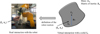 |
Fig. 2 Modeling of the virtual solid motion. |
3 Estimation of the operator forces
In the literature, two ways are used to determine the forces applied by the operator to the robot. The first one, which is less expensive, consists of estimating the applied forces using an analysis of the motor torque feedback and a dynamic model [21–23]. However, for applications requiring high accuracy or when the applied forces are relatively small compared with the inertia generated by the robot motion, a force sensor is mounted on the robot end-effector for a more accurate estimation [24–26]. In our case, a sensor is necessary due to the low value of the forces required to manipulate the tool in an intuitive way. Concretely, the situation corresponds to the experimental setup of Figure 3, which presents the co-manipulation of a probe. The force sensor is placed between the probe and the sixth axis of the robot.
The screw that collects the vector of measured forces fm and torques τm is denoted as  . This screw is deduced from the direct sensor measurement. It is the sum of the forces exerted by the operator
  , and the gravity and assembly forces
  due to the weight of the tool. The probe and the sensor-holder are modelled as a subsystem of mass ms. The forces read by the sensor can be defined by equation (11), where ps is the weight of the probe and the sensor-holder.
 (11)
(11)
where ds is the vector from point Om, the center of the force sensor, to point Gs, the probe center of gravity, and dm is the vector from point Om to point Oe.
In this way, the estimated forces  and
and  applied by the operator can be computed according to equation (12). Equation (13) presents the forces
  that are identified by an experimental process.
 (12)
(12)
 (13)
(13)
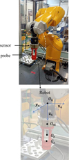 |
Fig. 3 Experimental system showing a probe attached to a 6-axis force sensor, mounted on the end effector of the Staübli TX2 60 robot. |
4 Synthesis
The generation of motion by the virtual solid method consists of calculating the trajectory of a virtual solid in a Galilean reference frame under the action of the operator forces. This instantaneous trajectory is sent to the robot numerical controller as an operating position set point. The calculation of the trajectory is done in three steps: the estimation of the handling forces from the measurements of a force sensor, their use in Newton’s second law to obtain the linear and angular accelerations of the virtual solid, and finally a double explicit numerical integration to compute the desired displacement corresponding to the applied forces. Figure 4 illustrates the diagram of the method.
The tuning parameters  are those that describe the virtual solid and the friction parameters. These parameters are all linked to a mechanical characteristic and behavior of the motion of the virtual solid. We can assume that the operator will intuitively tune them according to its feeling. If it has no knowledge of mechanical engineering, we could imagine developing experimental models to help it understand the impact of tuning parameters on the feel. For example, we could imagine a model with a solid moving in water and oil to identify the influence of viscous friction. Indeed, the virtual solid can be assimilated to the real tool manipulated by the operator without the robot and tool holder interaction. The physical parameters can be set, for the first time, as the inertia of the used tool with light frictions leading to a free move in the air. Then physical parameter tuning can be easily done by the operator: adjusting the inertia for the weight sensation, increasing the dry friction as a threshold for the low forces to avoid slow motion, and increasing the viscous friction to filter the vibration and avoid fast moves.
Stiffness control, impedance control, and our method are all based on a motion from the dynamics of a system. The main difference lies in the system definition (see Fig. 5). In the stiffness control case, the system is a mass-spring-damper, representing the interaction between the operator and the end-effector whose position is directly controlled. In the impedance control case, the system is a mass-damper, representing the interaction between the operator and the end-effector, whose position is indirectly controlled by the speed controller. In our case, the system is a virtual solid, representing the end-effector that should follow the operator’s desired trajectory. The fundamental equations of these three control laws are given in Table 1.
The tuning of the control parameters seems to be easier for the virtual solid method, since it refers to a physical movement. The dry friction parameter acts as a threshold on the motion without modifying the measured forces while maintaining a smooth motion. The viscous friction parameters function as a damping ratio. Moreover, the consistency of the co-manipulation behavior in translational and rotational motion is easy to achieve, since the mass and inertia parameters derive from the characteristics of the same solid.
The following sections present the simulation and experimental results obtained.
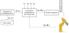 |
Fig. 4 Flowchart for determining the co-manipulation path using the virtual solid method. |
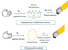 |
Fig. 5 Difference of behavior between stiffness control and virtual solid trajectory planning. |
Comparison between stiffness control, impedance control, and virtual solid control.
5 Simulation results
The use of simulation allows the exploration of numerous situations in a relatively short time. Thus, in order to study the behavior of the robot during manual guidance by the virtual solid method, the trajectory generation law is implemented under Simulink, a platform for multi-physics simulation and modeling of dynamic systems integrated with Matlab. For the tests, we worked with the Staübli TX2 60 robot, shown in Figures 2 and 3. So, the realization of the simulator requires establishing its Direct Geometric Model (DGM) and the Inverse Geometric Model (IGM) to simulate the position of the robot. The controller’s performance is not taken into account; thus, desired and actual velocities and positions are considered to be equal.
As illustrated in the block diagram in Figure 6, the trajectory generator receives as input the measured forces ( and
and  ) from the sensor, the current joint positions of the robot (q), and the current Cartesian velocity of the control point (
 and
and  ). The acceleration generator block calculates the desired acceleration of the co-manipulated point according to equation (8), from which the acceleration of point O6 and the angular acceleration of frame R6 are deduced. O6 is the center of the sixth axis of the robot and R6 is the frame attached to the sixth robot axis (Fig. 3). Then, the two integration blocks, respectively, calculate the velocity and the position of O6 and the angular velocity and orientation of frame R6. We present the results for both translational motion and rotational motion.
Thus, for all the tests, the virtual solid is considered to be cylindrical (similar to the ultrasound probe) with a height  , a base radius
  , and a virtual mass of
  . The friction values applied to the virtual solid, during each test, are presented in Table 2, where
  and
and  represent, respectively, the coefficients of dry and viscous friction in translation and
  and
and  those in rotation. We chose to set the dry friction coefficients to zero in the simulations because the applied force can be considered without noise. In reality, they generate only the minimum force required to set the robot in motion. These parameters are useful experimentally for the stability of the initial motion and its stopping. The viscous friction in rotation is also set to zero, as it is easier to illustrate the impact of dry friction on a tool path in translation.
The integrator saturation bounds consider the constraints of velocity inherent to the robot during the collaborative interactions, i.e. 250 mm.s−1, for each Cartesian axis in translation. As the rotational velocity limit is not normalized, we set it to 0.5 rad.s−1. The generation of motion in the operational space implies a transformation into articular coordinates of each point of the trajectory, which can fail when the computed trajectory passes through a singular position or when the computed point lies outside the working space of the robot. In this way, we have set the workspace according to the limits given in Table 3.
In order to evaluate the transparency of the motion at the handling point, we use two criteria proposed in the literature for a co-manipulated robot. The first one consists of studying the consistency between the applied forces and the effective displacement of the tool. According to Balhoul and Jlassi, the motion is transparent if equation (14) is verified [19,20]. This means that the force and the displacement are collinear and that their vectors have the same direction. The second criterion consists of analyzing the mechanical impedance at the interaction point. In fact, the higher the impedance, the more rigid the system is, and therefore the more difficult it is to manipulate the end-effector. The impedance matrix ( ) is calculated using equation (15). For this work, we are only interested in the diagonal elements of the impedance matrix, without taking into account the couplings. Thus, the vector of the diagonal of the impedance matrix, denoted
  , whose norm is computed in equation (16), represents the stiffness of the co-manipulation at the point
  .
.
 (14)
(14)
 (15)
(15)
 (16)
(16)
The obtained results are presented below.
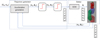 |
Fig. 6 Block diagram of the simulator. |
Friction table.
Limits of the workspace.
5.1 Flat translational motion with changes in motion direction
The forces  are applied progressively at
  by varying their direction, as illustrated by the force trajectory shown in Figure 7a. As only forces are applied, there is no rotation of frame
  . The simulator computes the acceleration (Fig. 7c), with a step of 1ms, and integrates it to find the corresponding velocity (Fig. 7b) and position of
  (Fig. 7d). Note that as the applied forces are low with a certain viscous friction that slows down the motion, the acceleration is very low except during sharp force direction change. For example, when force
  is suddenly null, as shown by equation (8), only the force due to viscous friction is not null and negative and has a high value due to the non-null velocity of the end-effector at this moment.
The analysis of the coherence between the applied forces and the effective displacement of point  gives the results displayed in Figure 8 and Figure 9.
As shown in Figure 8, the dot product remains greater than zero throughout the motion except at point a, so both vectors are in the same direction. Also, Figure 9 shows that the cross product values are almost negligible in the phases of rectilinear motion, on the order of 10-8, but non-negligible in the areas of direction variations, peaking at 10−3. Indeed, at the moment of the direction change on Figure 7 (between times t1 and t2 or t3 and t4), the velocity direction does not change at the same time as the forces. This is because the applied force direction change occurs when the velocity is not null, and friction parameters introduced in the trajectory generation computation generate a delay. Thus, at the time of the direction change of the applied forces, the system, already having a non-zero velocity, must first decelerate until total cancellation of the velocity before moving in the opposite direction. Friction promotes rapid deceleration but increases the acceleration time. This movement corresponds to the behavior of a solid moving according to Newton’s laws.
Also, Figure 10 shows the impedance at point Oe. At the beginning of the trajectory, it decreases in less than a second from 85 N/m.s-1 to approximately 5 N/m.s-1 and then stabilizes. Impedance is low, so the system is quite smooth. However, in the direction change area, the impedance oscillates weakly due to the friction phenomenon described above. The variation of the impedance indicates that in the direction change area, the operator can feel the inertia of the virtual solid, which is consistent with the human perception when handling everyday objects.
This feeling is stronger when the applied efforts and the speed of the controlled point are significant, as is the case at the point a of Figure 8 and Figure 10. Indeed, at this point, the probe moves in a direction opposite to the applied force for a short time. Note that, the motion is smooth only if the applied forces are also progressive and smooth.
A final analysis allows us to conclude concerning the co-linearity criterion: in the case of a circular motion of the virtual solid, as shown in Figure 11, the acceleration and the velocity are nearly orthogonal.
In addition, because of the frictional forces, the acceleration lags behind the forces by an α angle. This means that the velocity vector and the force vector are not aligned with an angle  . Thus, the criterion of transparency that consists of having the force and the velocity always collinear cannot be verified in the case of circular motion; it is valid only for rectilinear motion.
The result obtained in this section questions the criteria for transparency defined in literature as they ae not consistent with the mechanical principles of Newton’s laws.
The next result shows the trajectory generated for a rotational movement around a tool fixed point.
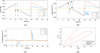 |
Fig. 7 Trajectories of force (a), velocity (b), acceleration (c), and position (d) of |

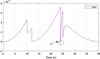 |
Fig. 8 Collinearity between forces and motions, dot product. |
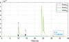 |
Figure 9 Co-linearity between forces and motions, cross product. |
 |
Fig. 10 Impedance graph during motion (left) and on the trajectory of Oe (right). |
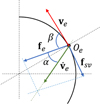 |
Fig. 11 Circular motion. |
5.2 Rotation around a fixed point
A torque of  defined in equation (17) is applied at Oe in order to create a rotation of the probe around the handling point Oe, as shown in Figure 12.
 (17)
(17)
The calculation of the impedance in rotation follows the same formula as in translation, replacing the forces with the torques and the translation velocity with the angular velocity. When the velocity in one direction is null, the diagonal component of the impedance matrix in this direction, resulting from equation (15), becomes infinite. However, as illustrated by the impedance norm curve resulting from equation (16), the impedance norm remains small, reflecting a smooth co-manipulation motion. Thus, these two different conclusions highlight the limitations of these two criteria in challenging the transparency of a control strategy.
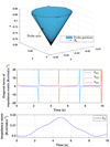 |
Fig. 12 Movement and impedance on a rotational motion. |
6 Experimental results
The trajectory generation by the virtual solid method is implemented on the Stäubli TX2 60 industrial robot and compared to the classical industrial method of robotic co-manipulation based on stiffness control for translational motions. We assume to only compare our method with a stiffness control, as both are based on position control law, contrary to the impedance control, which is based on velocity or force control law. Neither of these control laws is available on our standard industrial robot.
In order to measure the forces applied by the operator, a six-axis Schunk FTN GAMMA 65-5 strain gauge load cell is mounted on the robot. The experimental implementation required the creation of an application interfaced with the internal robot control, which we called Hand-Guidance. This application can be used either to implement a virtual solid or a stiffness co-manipulation method. It is the object of a registration at the Agence pour la Protection des Programmes (APP) in France.
The parameters of the virtual solid are the same as in simulation. The dry friction is set to 0.01 N and the viscous friction to 1 kg.s−1 in all directions. For the classical stiffness method, the stiffness of the system is fixed. The system is considered as a spring of stiffness k = 6 N.mm−1 in all directions in order to have a similar kinematic behavior to the virtual solid method.
The robot is set in motion to realize several go-to and return toolpaths of approximately 100 mm in a horizontal plane. Thus, we evaluate the forces deployed by the operator, the smoothness of the motion, and the robot’s influence on the obtained trajectory. Note that the operator tool trajectory is not the same for the two methods. The experimental results are obtained with random trajectories performed by the same operator. However, we observe equivalent results across multiple experiments with different operators. Note that the aim of the paper is to demonstrate the feasibility of virtual solid control and to highlight its potential benefits. The implementation of a stricter experimental protocol is considered as a perspective.
6.1 Handle force analysis
The manipulation forces during co-manipulation using the virtual solid method (denoted FeSV) and by the stiffness method (denoted FeR) are shown on the left in Figure 13, while the corresponding trajectories are shown on the right.
As shown in Figure 13, with the stiffness method, the operator must always apply forces on the probe. With the virtual solid method, the operator-applied forces are smaller, and sometimes they are null when kinematic variation is small. This behavior results from Newton’s second law, where the applied forces are directly linked to the tool acceleration. Thus, a motion can persist without an applied force. On the y0 axis for example, the maximum force in stiffness is nearly 10 N, while it is less than 5 N in virtual solid. The co-manipulation energy, expressed as the work of the manipulation forces on the experimental trajectories, for each co-manipulation method, is illustrated in Figure 14. As shown by the work curves, the operator provides more energy with the stiffness method than with the virtual solid method. Therefore, the proposed method enables a reduction of the manipulation forces.
We continue the comparative analysis by estimating the stiffness at the manipulated point Oe.
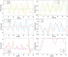 |
Fig. 13 Experimentally applied forces along the three Cartesian directions for each method (left) and the corresponding experimental trajectories along the three Cartesian directions (right). The index “R” denotes the stiffness method and the index “SV” denotes the virtual solid method. |
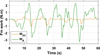 |
Fig. 14 Handling force work by the stiffness method (WR) and by the virtual solid Method (WSV). |
6.2 Analysis of stiffness at the manipulated point
By applying the equation (16), the impedance that reflects the stiffness of the manipulation is computed. The result for each method, presented in Figure 15, shows that the system is more rigid with stiffness than with virtual solid. Note that the peaks in the impedance graph, for both methods, are due to the phase of motion where the velocity is null or small, so the calculated numerical impedance tends to infinity, but this does not represent a real infinite stiffness.
We finish this section by showing that the motion obtained with the proposed method generates less jerkiness than that obtained with the stiffness method.
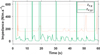 |
Fig. 15 Impedance calculated at the interaction point, for the two trajectory generation strategies. |
6.3 Analysis of shaking sensations
Milstein and Jarrasse propose analyzing velocity, acceleration, and jerk curves in order to evaluate the inertia of the manipulator and the disturbances perceived by the operator [27, 28]. The smoother the curves are, the less perceptible the shocks become. Figure 16 presents the velocity and acceleration trajectories of the manipulator point for the virtual solid method, while Figure 17 presents the velocity and acceleration profiles for the stiffness method for the motion and force trajectories shown in Figure 13. It can be observed in Figure 16 and Figure 17 that the acceleration profile is smoother in the case of the virtual solid method than in the stiffness method.
The trajectory generated by the proposed method is interesting because it allows the management of velocity and acceleration thresholds according to the operator’s needs. As acceleration and speed are computed simultaneously with position, the tool kinematics can be easily controlled without modifying the control law parameters.
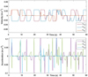 |
Fig. 16 Velocity and acceleration trajectories of the Oe point for the virtual solid method. |
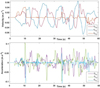 |
Fig. 17 Velocity and acceleration trajectories of the Oe point for the stiffness method. |
6.4 Robot influence on the trajectory generation
In order to visualize the robot influence on the trajectory generation, we compare the experimental trajectories from the previous tests with the theoretical trajectories computed by the simulator, based on the experimental forces measured by the sensor.
Figure 18 shows the results obtained for the virtual solid method. The components of the experimental trajectory of the robot are shown as a solid line in Figure 18 and are denoted as Xexp, Yexp, and Zexp. In simulation, for the same parameterized conditions as in experiment, we obtain the theoretical trajectories noted as Xth, Yth, and Zth, and illustrated with dashed lines. As shown in Figure 19, the theoretical position is ahead of the experimental position. This delay reflects the resistance of the robot to the experimental motion. Indeed, the structure of the robot opposes a resistance to the manipulation that must be taken into account during tuning. The friction values of the virtual solid control must be adjusted in order to avoid the influence of the robot on the actual generated tool path. Thus, the viscous friction whose experimental parameterization was 1 kg.s−1 increased to 2.5 kg.s−1 in simulation, making it possible to obtain the theoretical curves indicated primes (Xth, Yth, and Zth), which coincide with the experimental trajectories.
Similarly, for the generation of motion by the stiffness method, the theoretical trajectories are ahead of the experimental trajectories (Fig. 19). In order to take into account the resistance of the robot to the motion, we must introduce a friction parameter. In this case, to make the theoretical trajectories coincide with the experimental trajectories, the viscous friction should be up to 25 kg.s−1, which is ten times higher than the value parameterized for the virtual solid method.
Regarding the transparency, the trajectory followed by the robot does not correspond exactly to the trajectory of the virtual solid in the reference frame, due to the deviations generated by the robot. These deviations depend on multiple factors, including the mechanical structure of the robot, its size, and its weight. Thus, one solution to reduce these deviations is to use smaller robots. Another solution, in continuity with this work, is to integrate this gap into the tuning of the model used to generate the trajectory. In this way, the co-manipulation toolpath dynamics are limited, ensuring that the co-manipulation behavior remains consistent with Newton’s laws and is not disturbed by phenomena related to the robot. Consequently, the experimental trajectory would conform to the simulated trajectory.
To conclude this study, we examine the possible influence of the virtual solid method on the dynamics of the co-manipulated robot.
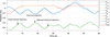 |
Fig. 18 Experimental and theoretical trajectories of the co-manipulated point Oe with the virtual solid method. |
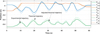 |
Fig. 19 Experimental and theoretical trajectories of the co-manipulated point Oe with the stiffness method. |
6.5 Trajectory influence on robot dynamics
In order to verify how the trajectory generation influences the robot dynamics, the joint torques of the robot are compared under the two trajectory generation strategies. Thus, the co-manipulation trajectories are presented in Figure 20, and the joint torques developed by the robot are illustrated in Figure 21. As shown in these figures, the torques developed by the robot with the virtual solid method evolve in the same way as those developed with the stiffness method. Trajectory generation using the virtual solid method does not affect the dynamics of the robot and therefore does not require any particular adjustment of the robot control system.
 |
Fig. 20 Experimental trajectories of the co-manipulated point Oe following the virtual solid method (left) and following the stiffness control (right) for the comparison of joint torques. |
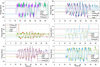 |
Fig. 21 Joint torques in co-manipulation by the virtual solid method and the stiffness control. With Fs identified dry friction of the robot joints. |
7 Conclusion
In this paper, we have analyzed a new trajectory generation approach for human–robot co-manipulation in order to improve the transparency and to simplify its tuning. As the trajectory followed by the robot corresponds to a solid motion in a Galilean reference frame, whose characteristics are similar to those of the co-manipulated tool, the manipulation of this tool should therefore appear transparent to the operator. The analysis of simulated and experimental results, based on the transparency evaluation criteria from the literature, showed that the virtual solid method generates smooth trajectories consistent with the operator’s intentions for any type of motion (translation and/or rotation). We have also demonstrated that compared to the classical implementation method, using the stiffness method, the virtual solid method enables robot co-manipulation with reduced manipulation efforts and does not require particular adjustments to the robot control. On the other hand, we have shown that the transparency criterion based on the collinearity between force and velocity is motion dependent and therefore not perfectly adapted to the transparency evaluation.
This work offers several perspectives. Indeed, we have seen that the presence of the robot affects the generated trajectory, but it is possible to significantly reduce the gap by tuning the viscous friction parameters. It would therefore be interesting to predict this deviation in order to tune the trajectory generation model and thus reduce the influence of the robot. It would also be relevant to study the parameters that influence the trajectory generation and to define a robust method for adjusting them according to the users and their perceptions. Firstly, the transparency of co-manipulation must be evaluated on technical gestures performed by users not familiar with the robot in order to collect their impressions of the interaction. Indeed, the first co-manipulation experiment was conducted with a clinician sonographer. It was found that when the sonographer co-manipulated the dummy probe without looking at the robot, the robot’s presence was almost imperceptible. However, when looking at the robot, the sonographer exerted much more effort and had the impression that the robot was disturbing the movement. Further experiments should be carried out in the same direction in order to draw conclusions and improve the acceptance of the robot's assistance. Moreover, the work in this paper only focused on the co-manipulation of the tool in the non-contact space. In the presence of contact, the trajectory generation law changes. In the future, it would be interesting to study the co-manipulation of the tool in contact with a surface. This would allow the development of an ultrasound gesture assistance system, in both position and force, with a compensation for the patient’s physiological movements.
Acknowledgments
We thank Maxime Humbert for his contribution to the experimental implementation of this work.
Funding
We would like to thank l’Agence Nationale des Bourses du Gabon for funding this thesis. Similarly, we thank the CRI program of CAP2025 and the Hub Innovergne which financially supported us and enabled us to acquire the force sensor essential for the experimental part of this work.
Conflicts of interest
The authors have nothing to disclose.
Data availability statement
The research data associated with this article are included in the article.
Author contribution statement
Conceptualization: I. Mousinga, F. Paccot, H. Chanal, and N. Bouton; Methodology: I. Mousinga, F. Paccot, H. Chanal, and N. Bouton; Software: I. Mousinga and F. Paccot; Validation: I. Mousinga, F. Paccot, H. Chanal, and N. Bouton; Writing—–Original Draft Preparation: I. Mousinga; Writing—–Review & Editing: I. Mousinga, F. Paccot, and H. Chanal; Supervision: F. Paccot, H. Chanal, and N. Bouton; Project Administration: F. Paccot and H. Chanal; Funding Acquisition: I. Mousinga, F. Paccot, and H. Chanal.
References
- F. Vicentini, Collaborative robotics: a survey, J. Mech. Des. 143, 040802 (2021) [Google Scholar]
- A. De Santis, B. Siciliano, A. De Luca, A. Bicchi, An atlas of physical human–robot interaction, Mech. Mach. Theory 43, 253–270 (2008) [Google Scholar]
- S. Haddadin, A. De Luca, A. Albu-Schaffer, Robot collisions: a survey on detection, isolation, and identification, IEEE Trans. Robot. 33, 1292–1312 (2017) [Google Scholar]
- A. De Luca, R. Mattone, Sensorless robot collision detection and hybrid force/motion control, in: Proceedings of the 2005 IEEE International Conference on Robotics and Automation, IEEE, Barcelona, Spain, 2005, pp. 999–1004 [Google Scholar]
- S.S. Jujjavarapu, A.H. Memar, M.A. Karami, E.T. Esfahani, Variable stiffness mechanism for suppressing unintended forces in physical human–robot interaction, J. Mech. Robot. 11, 020915 (2019) [Google Scholar]
- C. Yang, G. Peng, L. Cheng, J. Na, Z. Li, Force sensorless admittance control for teleoperation of uncertain robot manipulator using neural networks, IEEE Trans. Syst. Man Cybern. Syst. 51, 3282–3292 (2021) [Google Scholar]
- L. Peternel, N. Tsagarakis, D. Caldwell, A. Ajoudani, Robot adaptation to human physical fatigue in human–robot co-manipulation, Auton. Robots 42, 1011–1021 (2018) [Google Scholar]
- M. Bamaarouf, F. Paccot, L. Sarry, H. Chanal, Development of a robotic ultrasound system to assist ultrasound examination of pregnant women, IEEE Trans. Med. Robot. Bionics 6, 796–805 (2024) [Google Scholar]
- V. Villani, F. Pini, F. Leali, C. Secchi, Survey on human–robot collaboration in industrial settings: safety, intuitive interfaces and applications, Mechatronics 55, 248–266 (2018) [Google Scholar]
- L. Villani, J. De Schutter, Force control, in: B. Siciliano, O. Khatib, (Éds.), Springer Handbook of Robotics, Springer International Publishing, Cham, 2016, pp. 195–220 [Google Scholar]
- F. Caccavale, B. Siciliano, L. Villani, Robot impedance control with nondiagonal stiffness, IEEE Trans. Autom. Control 44, 1943–1946 (1999) [Google Scholar]
- N. Hogan, Impedance control: an approach to manipulation, in: 1984 American Control Conference, IEEE, San Diego, CA, USA, 1984, pp. 304–313 [Google Scholar]
- A.-N. Sharkawy, P.N. Koustoumpardis, Human–robot interaction: a review and analysis on variable admittance control, safety, and perspectives, Machines, 10, 591 (2022) [Google Scholar]
- A. Scibilia, M. Laghi, E. De Momi, L. Peternel, A. Ajoudani, A self-adaptive robot control framework for improved tracking and interaction performances in low-stiffness teleoperation, in: 2018 IEEE-RAS 18th International Conference on Humanoid Robots (Humanoids), IEEE, Beijing, China, 2018, pp. 280–283 [Google Scholar]
- S. Gopinathan, S.K. Ötting, J.J. Steil, A user study on personalized stiffness control and task specificity in physical human–robot interaction, Front. Robot. AI 4, 58 (2017) [Google Scholar]
- L. Peternel, N. Tsagarakis, A. Ajoudani, Towards multi-modal intention interfaces for human–robot co-manipulation, IEEE Int. Conf. Intell. Robots Syst., 2016, 2663–2669 (2016) [Google Scholar]
- P. Maurice, Y. Measson, V. Padois, P. Bidaud, Assessment of physical exposure to musculoskeletal risks in collaborative robotics using dynamic simulation, in: V. Padois, P. Bidaud, O. Khatib, (Eds.), Romansy 19 – Robot Design, Dynamics and Control. CISM International Centre for Mechanical Sciences, vol. 544., Springer, Vienna, 2013, pp. 325–332 [Google Scholar]
- D. Kushida, M. Nakamura, S. Goto, N. Kyura, Human direct teaching of industrial articulated robot arms based on force-free control, Artif. Life Robot. 5, 26–32 (2001) [Google Scholar]
- S. Jlassi, S. Tliba, Y. Chitour, An event-controlled online trajectory generator based on the human–robot interaction force processing, Ind. Robot Int. J. 41, 15–25 (2014) [Google Scholar]
- A. Bahloul, Sur la commande des robots manipulateurs industriels en co-manipulation robotique, Université Paris-Saclay, (2018) [Google Scholar]
- S. Zhang, S. Wang, F. Jing, M. Tan, A sensorless hand guiding scheme based on model identification and control for industrial robot, IEEE Trans. Ind. Inform., 15, 5204–5213 (2019) [Google Scholar]
- S.-D. Lee, K.-H. Ahn, J.-B. Song, Torque control based sensorless hand guiding for direct robot teaching, in: 2016 IEEE/RSJ International Conference on Intelligent Robots and Systems (IROS), IEEE, Daejeon, South Korea, 2016 [Google Scholar]
- H. Sang, J. Yun, R. Monfaredi, E. Wilson, H. Fooladi, K. Cleary, External force estimation and implementation in robotically assisted minimally invasive surgery, Int. J. Med. Robot., 13, e1824 (2017) [Google Scholar]
- A. Winkler, J. Suchý, Force-guided motions of a 6-d.o.f. industrial robot with a joint space approach, Adv. Robot. 20, 1067–1084 (2006) [Google Scholar]
- D. Kubus, T. Kroger, F.M. Wahl, Improving force control performance by computational elimination of non-contact forces/torques, in: 2008 IEEE International Conference on Robotics and Automation, IEEE, Pasadena, CA, USA, 2008, pp. 2617–2622 [Google Scholar]
- E. Mariotti, E. Magrini, A.D. Luca, Admittance control for human–robot interaction using an industrial robot equipped with a F/T Sensor, in: 2019 International Conference on Robotics and Automation (ICRA), IEEE, Montreal, QC, Canada, 2019, pp. 6130–6136 [Google Scholar]
- A. Milstein, T. Ganel, S. Berman, I. Nisky, human-centered transparency of grasping via a robot-assisted minimally invasive surgery system, IEEE Trans. Hum. Mach. Syst. 48, 349–358 (2018) [Google Scholar]
- N. Jarrasse et al., A methodology to quantify alterations in human upper limb movement during co-manipulation with an exoskeleton, IEEE Trans. Neural Syst. Rehabil. Eng. 18, 389–397 (2010) [Google Scholar]
Cite this article as: I. Moutsinga, F. Paccot, H. Chanal, N. Bouton, Analysis of a new reactive control strategy to improve transparency of human-robot co-manipulation, Mechanics & Industry 27, 7 (2026), https://doi.org/10.1051/meca/2026008
All Tables
Comparison between stiffness control, impedance control, and virtual solid control.
All Figures
|
Fig. 1 Stiffness or impedance control behaviur. |
| In the text | |
|
Fig. 2 Modeling of the virtual solid motion. |
| In the text | |
|
Fig. 3 Experimental system showing a probe attached to a 6-axis force sensor, mounted on the end effector of the Staübli TX2 60 robot. |
| In the text | |
|
Fig. 4 Flowchart for determining the co-manipulation path using the virtual solid method. |
| In the text | |
|
Fig. 5 Difference of behavior between stiffness control and virtual solid trajectory planning. |
| In the text | |
|
Fig. 6 Block diagram of the simulator. |
| In the text | |
|
Fig. 7 Trajectories of force (a), velocity (b), acceleration (c), and position (d) of |
| In the text | |
|
Fig. 8 Collinearity between forces and motions, dot product. |
| In the text | |
|
Figure 9 Co-linearity between forces and motions, cross product. |
| In the text | |
|
Fig. 10 Impedance graph during motion (left) and on the trajectory of Oe (right). |
| In the text | |
|
Fig. 11 Circular motion. |
| In the text | |
|
Fig. 12 Movement and impedance on a rotational motion. |
| In the text | |
|
Fig. 13 Experimentally applied forces along the three Cartesian directions for each method (left) and the corresponding experimental trajectories along the three Cartesian directions (right). The index “R” denotes the stiffness method and the index “SV” denotes the virtual solid method. |
| In the text | |
|
Fig. 14 Handling force work by the stiffness method (WR) and by the virtual solid Method (WSV). |
| In the text | |
|
Fig. 15 Impedance calculated at the interaction point, for the two trajectory generation strategies. |
| In the text | |
|
Fig. 16 Velocity and acceleration trajectories of the Oe point for the virtual solid method. |
| In the text | |
|
Fig. 17 Velocity and acceleration trajectories of the Oe point for the stiffness method. |
| In the text | |
|
Fig. 18 Experimental and theoretical trajectories of the co-manipulated point Oe with the virtual solid method. |
| In the text | |
|
Fig. 19 Experimental and theoretical trajectories of the co-manipulated point Oe with the stiffness method. |
| In the text | |
|
Fig. 20 Experimental trajectories of the co-manipulated point Oe following the virtual solid method (left) and following the stiffness control (right) for the comparison of joint torques. |
| In the text | |
|
Fig. 21 Joint torques in co-manipulation by the virtual solid method and the stiffness control. With Fs identified dry friction of the robot joints. |
| In the text | |
Current usage metrics show cumulative count of Article Views (full-text article views including HTML views, PDF and ePub downloads, according to the available data) and Abstracts Views on Vision4Press platform.
Data correspond to usage on the plateform after 2015. The current usage metrics is available 48-96 hours after online publication and is updated daily on week days.
Initial download of the metrics may take a while.