


| Issue |
Mechanics & Industry
Volume 27, 2026
A French vision of advances and prospects in mechanics: industry, research and training needs
|
|
|---|---|---|
| Article Number | 26 | |
| Number of page(s) | 41 | |
| DOI | https://doi.org/10.1051/meca/2026022 | |
| Published online | 11 June 2026 | |
Review
Computational mechanics empowered by artificial intelligence
1
PIMM, Arts et Metiers Institute of Technology, Paris, France & CNRS@CREATE, Singapore
2
Université Paris-Saclay, CentraleSupélec, ENS Paris-Saclay, CNRS, LMPS - Laboratoire de Mécanique Paris-Saclay, Gif-sur-Yvette, France
3
Univ Toulouse, IMT Mines Albi, INSA Toulouse, ISAE-SUPAERO, CNRS, ICA, Albi, France
4
Institut Jean Le Rond d'Alembert, Sorbonne Université, CNRS, Paris, France
5
SafranTech, France
* e-mail: This email address is being protected from spambots. You need JavaScript enabled to view it.
Received:
15
December
2025
Accepted:
15
April
2026
Abstract
The present paper revisits recent challenges in computational mechanics where data-driven modeling offers unexpected possibilities. For that purpose, the main concepts related to data and learning are first introduced. Then, physics-based, data-driven, and hybrid modeling approaches in the different domains of mechanics: solids and structures, fluids and flow, and processing and manufacturing will be addressed. Finally, technology needs, recent advances, and remaining challenges in the industrial sector will be highlighted.
Key words: Computational mechanics / hybrid modeling / data-driven solid mechanics / data-driven fluid mechanics / data-driven manufacturing
© F. Chinesta et al., Published by EDP Sciences, 2026
 This is an Open Access article distributed under the terms of the Creative Commons Attribution License (https://creativecommons.org/licenses/by/4.0), which permits unrestricted use, distribution, and reproduction in any medium, provided the original work is properly cited.
1 Introduction
The last century was prolific in achievements in almost all the domains of engineering. Engineering models found a major ally in applied mathematics, which, from a panoply of advanced discretization techniques and the use of powerful computational platforms, enabled the solutions of the sophisticated mathematical problems describing the observed reality.
These problems usually take the form of coupled nonlinear partial differential equations describing, in general, the multiphysics and multiscale character of the phenomena under scrutiny. They resulted from centuries of scientific discovery, guided by reasoning, complemented by inspiration, creativity, and intuition, shaping the so-called art of modeling that characterizes modern physics. That guided reasoning characterizing scientific discovery operated on the measurements performed on the observed reality, because a model is no more than the link between actions (input) and consequences (output).
In the domain of traditional modeling, almost human-centric, the technical difficulties related to the data acquisition and ulterior manipulation to distill the searched model induced, in general, a long process.
However, the 21st century represented a new revolution concerning both (i) the engineering expectations and (ii) the disruptive technologies at hand. With regards to the engineering domain, some major challenges appeared induced by the advent of unprecedented technological necessities:
The need to scale up, moving from the well-mastered component scale to that of complex systems of systems;
The need to move from traditional design toward efficient operation, requiring predictions that are both fast and accurate;
Design should escape from the too constrained design space, in general, parametric, to unbounded design domains, if possible, non-parametric, to reach disruptive design capabilities.
These opportunities implied conceptual, theoretical, and practical challenges.
First, moving from the component level to the system level implies not only an increase in problem size but, more importantly, the propagation of inaccuracies or uncertainties, compromising predictions and reducing the prediction horizon (in space and time). In most cases, complex systems, even when carefully modeled without considering computational cost, exhibit a gap between observation and prediction. This gap, referred to here as ignorance, represents the part of reality that is absent from the considered model.
Second, in the past, fast and accurate were usually pushing in opposite directions. When looking for rapidity, models were generally degraded, with the associated loss of accuracy. On the other hand, when looking for extreme accuracy, the simulation time became prohibitive, excluding its use in real-time control applications.
1.1 Four modeling paradigms
Four major modeling paradigms can be distinguished, as summarized below:
Within the physics-based modeling (PBM) setting, models describing the phenomena under scrutiny are assumed available. These models can nowadays be solved by using appropriate discretization techniques, most of them available in commercial simulation software. Despite the impressive achievements that this framework made possible in sciences and engineering, two major difficulties persist: (i) the lack of accuracy when addressing very large simulations in space and time, due to the propagation of modeling inaccuracies and uncertainties, as well as, in some cases, incomplete knowledge of the observed reality; and (ii) the computational cost (CPU) and computational resources to be deployed.
Within the data-driven modeling (DDM) setting, the model is learned from available data by using an appropriate machine learning technique. Here, we assume available data consisting of inputs and the associated outputs, from which a model, able to connect the output to the corresponding input, is constructed. The just-learned model can then be applied to infer the output associated with a given input (direct problem) or to identify the input related to an observed output (inverse problem). Thus, in principle, only data and appropriate machine learning techniques seem to be needed to construct the model. Despite its simplicity and generality, some issues persist, among them: (i) the amount of data needed for constructing the model, which strongly depends on the data modality under consideration (e.g., scalar data, time series, images, full fields, graphs, or simulation databases), as well as on the level of embedded physical knowledge; (ii) the data acquisition itself: which data, at which scale, where and when collecting it, etc.; (iii) the extrapolation issue when applying the learned model far from the learning domain; and (iv) the difficulty to explain both the model itself and the decision resulting from its application, which makes certifying difficult engineering, with the associated impact on its industrial and societal adoption.
Within the physics-informed learning (PIL) setting, the resulting learned model becomes a compromise between existing knowledge, for instance, a model expected to represent the first order of the observed reality, and data, both contributions weighted according to the degree of confidence in each contribution. Because of the knowledge incorporation, the amount of data reduces significantly, while the resulting learned model becomes much more explainable and is therefore easier to certify.
Finally, within the physics-augmented learning (PAL) setting, the observed reality is assumed to exhibit a gap with respect to the predictions from a good state-of-the-art physics-based model. Machine learning is then applied to that gap, the so-called ignorance, in order to model it. When adding the model of ignorance to the physics-based model prediction, the observed reality is expected to be accurately approximated. When the first-order model is good enough and then the ignorance is quite small, the amount of data needed for improving (enriching or correcting) the model reduces significantly. Again, the enriched model gains in explainability, which is of critical interest in engineering.
1.2 Four main levels of digitalization
After three industrial revolutions induced by the steam, electricity, and electronics (with its associated automation), the so-called fourth revolution concerned the use of data to create digital replicas. In that sense, four levels of digitalization can be distinguished:
For a designer interested in the shape of a new design, its CAD description represents a valuable twin that virtually replicates from the geometrical and aesthetic point of view the searched design.
However, in general, in engineering, other than the shape and aesthetic, the performance is of major interest. To evaluate it, the geometry must be complemented with physics, the one governing the response of the design under the potential applied actions. This level of digitalization is known as numerical simulation. It was and continues to be nowadays a major protagonist in science and engineering.
The previously mentioned twins precede the existence of the physical system and constitute the so-called twin prototype, of crucial interest in the phase of design. As soon as the physical system is manufactured, it could be operated, with its digital twin replicating its behavior and then facilitating its optimal operation. Its main function is to mirror and predict the functioning and performance throughout the entire life cycle of the associated physical system. Its three main components are (i) the physical system equipped with the appropriate sensors and actuators; (ii) the communication networks (e.g., IoT and 5G) enabling the data transfer from the sensors to the virtual replica of the physical system (monitoring) and from the virtual replica to the actuators (control); and (iii) the virtual replica itself, which at its turn consists of the best physics-based and/or data-driven model emulating the system behavior with the greatest accuracy while performing under the stringent real-time constraint.
When the just-described digital twin operates, its accuracy continuously improves because it learns continuously from the acquired and digested data. However, when many similar assets coexist in a larger system, each could benefit from the others, constituting the so-called digital twin aggregate.
Thus, digital twins seem well aligned with the two main missions of engineers and engineering: (i) design, facilitated by the digital twin prototype; and (ii) operation, facilitated by the digital twin instance and aggregate.
2 About data
2.1 Data and its typology
Data do not admit a unique intrinsic definition. Rather, a dataset is composed of features whose nature depends on the intended use. In a simple mechanical test, for instance, a data point may consist of an applied force and the associated specimen extension. In such a case, the force plays the role of an input feature when learning a model for the extension.
In some situations, data are not naturally represented in a Euclidean vector space. Measuring similarity or proximity between data points then requires not only a representation but also an appropriate metric.
The most common typologies of data are (i) lists or tabulated data, involving continuous or discrete numerical values, categorical features, etc.; (ii) images (structured 2D or 3D images) or numerical simulation fields that can be viewed as non-structured images, better represented as graphs; (iii) tensor formats, describing compressed images or data; (iv) graphs; and (v) curves and time-series, the latter similar to curves but constrained by causality.
2.2 Data reduction
Given the subtle nature of data, a major issue is the selection of the features that each data point should involve: no more than needed for the modeling purpose, but no less either.
Feature reduction can be performed by statistical analysis or by dimensionality reduction techniques aimed at identifying a lower-dimensional manifold supporting the data. The corresponding intrinsic dimensionality reflects the effective number of independent degrees of freedom needed to represent the dataset.
Dimensionality reduction techniques can be linear or nonlinear. Among the different linear reduction techniques, principal component analysis (PCA) [1] is widely applied. Among the nonlinear techniques, locally linear embedding (LLE) [2], kernel principal component analysis (kPCA) [1], local principal component analysis (ℓ-PCA), multidimensional scaling (MDS) [1], t-distributed stochastic neighbor embedding (t-SNE) [3], among others, are widely considered.
Autoencoders (AE), employing neural network (NN) architectures, represent an alternative route to nonlinear dimensionality reduction, are very efficient, operating in a quite transparent way, and enabling direct and inverse mappings [4–6].
Among the many available techniques, PCA, LLE, and AE are briefly discussed below, as they illustrate the main ideas underlying linear and nonlinear dimensionality reduction. In what follows, the generic high-dimensional data point is denoted by  .
.
2.2.1 Linear dimensionality reduction: the principal component analysis—PCA
Let  denote a data vector expected to lie close to a d-dimensional manifold with d ≪ D.
PCA considers the linear transformation defined by the orthonormal matrix W, with  (identity matrix of size d), such that
  . Data yi and ξi, 1,...,M (both assumed centered) define the columns of matrices Y and Ξ respectively. PCA looks for a maximal variance and decorrelation in the latent variable set ξ.
The covariance matrix  (where
  refers to the statistical expectation) can be factorized as
  . Thus,
  . By pre- and post-multiplying by WT and W respectively, it results
  or
or  , where
  becomes diagonal if
  , i.e., W is composed by the d eigenvectors associated with the d non-zero eigenvalues of matrix Cyy, that represent the variance of the latent variables ξ.
2.2.2 Nonlinear dimensionality reduction: locally linear embedding-based manifold learning—LLE
Given data points  ,
,  , LLE proceeds in two steps [2]:
First, a linear interpolation of each data point
 ,
,  is performed from its K nearest neighbors, K being a hyper-parameter:
  (the set Si containing the yi K-nearest neighbors). LLE then computes the approximation weights Wij by minimizing the functional
  .
.Each patch consisting of neighboring data points around yi,
 , is mapped onto a space of dimension d ≪ D while keeping the just computed interpolation weights. The corresponding coordinates
  (associated with yi) and having the same neighbors are computed by minimizing the functional:
  .
.
2.2.3 Nonlinear dimensionality reduction: autoencoders—AE
The just-discussed nonlinear dimensionality reduction techniques successfully achieve data reduction, moving from  to a d-dimensional (d ≪ D) manifold, but generally fail to perform the inverse mapping, i.e., finding y(ξ). The so-called AE [4–6] represent a valuable alternative to learn both the data reduction (encoder) as well as the inverse mapping (decoder).
The high-dimensional data  is nonlinearly mapped (from the use of a neural network) into the so-called latent space, consisting of a hidden layer composed of d neurons, as before assuming d ≪ D, leading to
  , the reduced counterpart of y, that the nonlinear decoder (a second neural network) expands to recover
  , as close as possible to y.
The minimum value of the hidden layer size (d) that enables to recover the original data by encoding and subsequent decoding, without an irreversible loss of information, represents the intrinsic data dimensionality. The associated data ξ is expected to be free of any (linear and nonlinear) correlation.
Assuming both the encoder and the decoder are two trainable neural networks,  and
and  , with parameters θe
and θd
respectively, the AE training can be expressed from
, with parameters θe
and θd
respectively, the AE training can be expressed from
 (1)
(1)
To increase efficiency, avoid overfitting, and reduce the amount of data employed in training, different regularizations were proposed, giving rise to the so-called sparse AE and other variants (variational, denoising, and contractive, among many other choices) [4,7,8].
2.3 Data clustering and classification
2.3.1 k-means based unsupervised data clustering
k-means is one of the most widely used unsupervised clustering techniques [9,10].
The M available high-dimensional data  ,
,  is distributed into k sets (k ≤ M),
  , in such a way that each member of a cluster is closer to the mean value of its cluster than to the mean value of any other clusters. This condition reads:
 (2)
(2)
where μi represents the i-cluster mean value.
On the other side, supervised classification considers labeled data in  , with the objective of finding the frontiers between the different data classes.
2.3.2 Support vector machine-based classification—SVM
Linear support vector machines (SVMs) seek hyperplanes that maximize the margin, which is the distance between the hyperplanes and the data, thereby increasing classification robustness. Nonlinear SVMs proceed similarly but employ kernels [11].
With the data labels zi and  representing two classes in the data:
  linear SVM looks for the hyperplane
  (w being the unit vector normal to the hyperplane), separating the data into two sets while maximizing the margin.
The distance between the hyperplanes defined by  is
is  . Thus, the margin maximization implies minimizing ||w||, with the separation constraint
 (3)
(3)
With both w and b calculated, the classifier becomes:
 (4)
(4)
2.3.3 Decision trees and random forest-based classification
A decision tree consists of nodes and branches [12]. Data are divided into two branches at each node, depending on the response to an appropriate question: true or false. Thus, the problem reduces to finding the right question formulated at the right moment. For that purpose, a grade of the so-called impurity is attached to each node.
The impurity is calculated at each node, before and after separation, whose difference leads to the so-called information gain. By comparing the information gain associated with each possible question, the one providing the maximum information gain becomes the optimal one.
If we consider different smaller datasets consisting of M ′ < M data points, randomly chosen, a set of trees results, the so-called forest [13]. If a new data point y is evaluated by using each tree and the classification predicted by each tree computed the random forest classification consists of the class that obtains the biggest number of votes for the ensemble of trees.
2.4 Data transformation
Sometimes features are associated with observable and measurable quantities. However, these features, very pertinent from the point of view of the technician, are much less pertinent from the point of view of the modeler. For example, measurable density, viscosity, and velocity result in the so-called Reynolds number, which is the only important parameter from the point of view of the flow model.
Moreover, the complexity of a learned model depends on the chosen observables. Describing the planet’s movement around the sun seems simpler than describing the universe with respect to the Earth, a very old concern!
Kernel-based PCA (kPCA) maps the data into a high-dimensional space in such a way that in that space the transformed data become embedded into a linear manifold, facilitating a linear dimensionality reduction (PCA). The difficulty of constructing such a mapping was replaced by the use of the so-called kernels to express the scalar product in the high-dimensional space from a kernel calculated in the original space [1].
This rationale was further developed with the introduction of AE, which facilitated the construction of such linearizing mappings, thereby avoiding the arbitrary choice of a kernel (the so-called kernel trick). This was the rationale followed in the development of the so-called rank reduction autoencoder (RRAE) described later, but it is also the one behind the use of AE within the Koopman theory [14, 15] to map the data of a dynamical system into a space in which the dynamics become linear.
2.4.1 Topological data analysis—TDA
Another valuable transformation consists of the use of topological data analysis (TDA) based on the persistence homology. It becomes an appealing alternative for describing data with huge topology content [16, 17]. This is the case for time series or images of microstructures (e.g., foams, polycrystals, and composite materials) [18–21]. TDA offers compact and concise metrics able to discriminate complex data from its intrinsic topology, to complement more experienced routes making use of statistical descriptors (e.g., statistical moments, pair-correlation, and covariogram [22]), on which applying learning strategies discussed later [18].
It is also well known that data could be transformed in such a way that their description becomes sparser. The elementary function cos(ωx) can be expressed in the Fourier space in a very compact manner. This rationale is at the origin of the so-called compressed sensing, of interest in signal analysis but also in some computational physics applications [23].
2.4.2 Compressed sensing in a nutshell
Let f be a vector, in the space or time domains, and c be its vector counterpart in a domain in which its representation is expected to be sparser. These spaces are in general related to frequency (Fourier or discrete cosine transforms) or to multi-resolution wavelets, among others, both expressions being related by the linear operator whose discrete expression consists of the matrix T, with Tc = f.
As c is expected to have many zero entries, few rows of T and vector f should suffice. For that purpose, an extraction matrix, E, defined as  and
and  , can be applied on the original linear system, leading to
  , which becomes underdetermined, and then having an infinite number of solutions.
In order to enforce the sparse character, i.e., the knowledge that most of the components of vector c are zero, it suffices to solve the underdetermined problem by employing a L1-norm based optimization, making use of LASSO for instance [23].
2.5 Toward data generation
Generative adversarial networks (GANs) and AE are appealing choices for generating new data from the one that served to train their respective involved neural networks.
2.5.1 Generative adversarial networks—GANs
GANs [24] are trained to differentiate real data from generated data. It contains two NN, the first called generator and the second discriminator. The generator tries to mislead the discriminator and be the last to unveil the data created by the generator.
The generator generates random inputs from a latent space while computing its parameters θG from the gradient of its cost function JG . At its turn, the discriminator uses as input the real data as well as the one generated by the generator to optimize its parameters θD to discriminate true and false data by diminishing its associated cost function JD .
The true and generated data are noted, respectively, by x and G(z), labeled, respectively, with 1 and 0, then the discriminator tries to produce D(x) = 1 and  respectively. The usual discriminator loss reads
 (5)
(5)
where  refers to the expectations of the true and generated data distributions.
Concerning the generator, its cost function could consist of  , even if an alternative widely employed reads
 (6)
(6)
Thus, when considering a sampling consisting of m true data xi,  , and m generated data G(zi),
  , the gradients considered in the training read
 (7)
(7)
2.5.2 Variational autoencoders—VAE
Variational autoencoders [7,25] encode data as probability distributions, thereby learning a continuous latent representation from which new samples can be generated in a more robust manner. Normal distributions are commonly considered in such a way that the encoder is trained to return the mean and the covariance matrix, both depending on the input data, which allows a statistical sampling on which the decoder applies.
The loss function considered in the network training is composed of two terms, the first enforcing data reconstruction and the second enforcing that the encoded distribution approaches a standard normal distribution. Covariance close to the identity prevents punctual distributions, and a mean close to zero ensures proximity. The most natural way of expressing that regularization consists of using the Kullback–Leibler divergence, which quantifies the discrepancy between two probability distributions, here the learned latent distribution and a prescribed reference one, typically a standard normal distribution in the VAE setting [26].
2.5.3 Rank reduction autoencoder—RRAE
Usual autoencoding, despite the data reduction performances, finds difficulties in performing robust generation and accurate interpolation. The latter is crucial for performing regression, as discussed later in the present paper.
If one provides circles to an AE, with the objective of generating others and eventually extracting the optimal one, a natural procedure could consist of the following:
Recognizing that the presented images consist of circles, which can be represented by a single parameter, their radius, for instance.
Then, the generation consists of selecting many values of that parameter in a given interval and drawing the associated circles.
If a cost function is applied to each, the circle minimizing it could be selected to represent the optimal design.
The procedure seems trivial as soon as one is able to recognize a way of parametrizing the concerned geometries. However, for arbitrary shapes, the situation becomes much less trivial, and one could be tempted to provide those arbitrary shapes to an AE to analyze their representation at its latent layer. In the case of the circles discussed above, the AE will discover that the initial images consisting of D pixels can be embedded into a one-dimensional space and then recovered as soon as the decoder is applied.
The original data are noted by xi,  , whereas its reduced counterpart in the one-dimensional latent space is noted by
  ,
,  .
.
Now, if we generate new values of y by interpolating from yi, the resulting geometries after decoding x(y) are not the expected intermediate circle as Figure 1 illustrates. The reason is that in the case of nonlinear reduced-order manifolds, a simple interpolation generates data outside the manifold, for which the decoder fails to provide an accurate circle.
To circumvent this issue, efforts should be made at the level of the latent space, concerning the representation or its interpolation. As discussed before, VAE enforced a particular structure of the hidden space to limit this issue; however, its training is, in general, very expensive and needs a significant amount of data.
The so-called rank reduction autoencoder (RRAE) [27], depicted in Figure 2, enforces a latent linear vector space, constraint easy to enforce by inserting a PCA layer in between the encoder and the decoder. It is important also to mention that here the data size increases, with the size of y larger (in general) than the one of the original data x, however this high-dimensional data are embedded into the low-dimensional PCA manifold.
Thus, the departure data x is encoded into the latent space, as a series of coefficients  (R being the reduced dimension of the latent space) associated with the corresponding orthonormal vectors
  , with the representation
 (8)
(8)
where the reduced coordinates αi can be computed easily, taking into account the basis orthonormality, that is
 (9)
(9)
In such a linear latent space, interpolation between two reduced representations  and
and  can be performed directly by considering
 (10)
(10)
before decoding y(λ) to obtain the corresponding interpolated data in the original space.
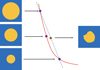 |
Fig. 1 Interpolation risks that could be incurred when operating in nonlinear manifolds. |
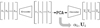 |
Fig. 2 Rank reduction autoencoder. |
3 About learning
3.1 Linear regressions
3.1.1 Polynomial approximations
If one looks for expressing a Quantity of Interest (QoI) y as a function of a number of variables xi,  , regressions based on polynomial approximations seem a natural choice
 (11)
(11)
approximation that becomes linear by considering only the linear terms related to β0 and βi,  , and nonlinear by considering quadratic and higher degree terms.
This approach represents a good choice in the case of (i) the QoI exhibiting a smooth polynomial behavior; (ii) the number of variables (features) P remains small enough and the interaction between the different features involves low-degree polynomial terms.
Thus, in general, the multiparametric case represents a challenge for usual polynomial approximations, because the enormous number of involved terms will need an enormous amount of data to compute the different involved β-coefficients.
To operate in multi-dimensional settings, separated representations constitute an appealing choice. These representations were largely employed in the so-called proper generalized decomposition (PGD) [28–31]. Such separated representations are constructed by computing sequentially the approximation in each dimension while keeping all the others frozen, within an alternating-directions fixed-point algorithm.
Thus, with all the data available to approximate each dimension, richer approximations can be envisaged; however, considering the problem globally, it could become underdetermined (exhibiting an infinite number of solutions), needing suitable regularizations to reconcile few data with rich nonlinear approximations in multidimensional settings while avoiding overfitting.
3.1.2 Regularized polynomial approximations
A first attempt to construct surrogates in high-dimensional settings, the so-called sparse subspace learning (SSL) [32], considers hierarchical orthogonal bases and their associated Gauss-Lobatto nodes, exhibiting excellent performance but requiring special treatment when the dimension increases too much.
To alleviate the issue just referred to, the authors in [33] proposed enriching the approximation in each dimension sequentially while increasing the polynomial degree used to approximate the different terms in the separated representation.
More robust regularizations made use of sparsity, inspired by the so-called sparse identification nonlinear dynamics (SINDy) regression [34]. SINDy uses a large dictionary of functions and then selects the sparsest approximation within the dictionary by penalizing the number of non-zero coefficients affecting the dictionary functions.
This regularization was then considered in [35], where separated representations were considered for performing in high-dimensional settings. Different regularizations were evaluated, e.g., Elastic-Net, Ridge, and Lasso. Another appealing technique also analyzed in [35] consisted of combining the anchored-ANOVA [36] for the linear terms without feature interaction, profiting from the variance analysis that the ANOVA provides [37], with a sparsely regularized polynomial for the terms involving feature interaction.
3.2 Nonlinear regressions
When the response manifold becomes more complex and more data are available, nonlinear regression techniques become more appropriate, especially those based on Neural Networks (NN) [4]. Their main advantages lie in their expressivity and flexibility, whereas their main limitations concern data requirements and interpretability.
The universal approximation theorems introduced for approximating functions [38] and the variants concerning functionals and operators ([39] and [40], respectively) explain the popularity of such techniques. NN can assimilate almost any typology of data, with images and graphs processed by using convolution [41].
To briefly recall the principle of a neural network, consider first a single neuron receiving two inputs, x1 and x2, and producing one output y.
The simplest option consists of performing a linear combination affecting each input with a weight, in our case, W1 and W2:  .
.
In the case of a neuron receiving P inputs, the weighted output results
 (12)
(12)
whose matrix form reads
 (13)
(13)
However, before employing Equation (13), the weights composing vector W must be calculated. This stage represents the so-called network training. To calculate the P weights, data are needed. If we assume the existence of M data, preferably with M > P:  , the weights can be determined from a quadratic minimization problem, whose specific form depends on the statistical properties of the measurement noise:
 (14)
(14)
with  and
and  . Equation (14) corresponds to a least-squares formulation, which is optimal under the assumption of Gaussian noise. More generally, the choice of the loss function reflects assumptions on the noise statistics. When the noise covariance is known, the optimal metric corresponds to a weighted quadratic form (Mahalanobis distance), whereas alternative robust losses (e.g., Huber-type) may be preferred in the presence of non-Gaussian noise or outliers [42].
However, until now, the setting remains linear. To enlarge its applicability domain, a nonlinear function, the so-called activation function  , emulating the fact that biological neurons only activate for large enough activations, is introduced to affect the neuron output
 (15)
(15)
whose training now considers the minimization problem expressed by
 (16)
(16)
When considering many neurons, many layers, and larger-size inputs and outputs, the rationale remains the same, and the specific architecture needs the determination of the network parameters (weights) and also the choice of the number of layers and neurons in each (the so-called hyperparameters). Concerning the choice of the activation function  , there are also many choices, and some choices enable preserving or ensuring some properties in the output (e.g., positivity and convexity).
3.3 Dynamical systems
In dynamical systems, the objective is to predict the time evolution of the state. Several strategies can be considered depending on the dimensionality of the state, the amount of available data, and the desired level of physical structure in the learned model.
3.3.1 Reduced dynamics
When the system state is very high-dimensional, for example, when it corresponds to a field defined over a 2D or 3D domain, a first strategy consists in constructing a reduced representation and then learning the associated reduced dynamics.
Imagine that the system state is known at times  , noted by
  . By introducing these states into the RRAE, a number of modes are extracted
  , where the reduced state y can be expressed from them:
 (17)
(17)
The reduced state evolution yn,  enables calculating
  ,
,  and
and  . Thus, for each mode i, the dynamical system governing the time evolution of αi could be extracted using one of the technologies described later.
3.3.2 Linearizing dynamics from dynamic mode decomposition – DMD
By assuming a uniform time stepping Δt, with  ,
,  , DMD [43] assumes the existence of a constant matrix B, such that
  ,
,  .
.
From the available data, the matrix B can be computed by operating with the state or with its reduced counterpart and enforcing in its construction the integration stability constraints [44].
This framework can be adapted for control purposes or for addressing nonlinear dynamics, assumed to be locally linear [45]. Nonlinear extensions can also be constructed by warping the snapshots into a higher-dimensional space spanned by suitably chosen nonlinear features so that the dynamics become approximately linear in that lifted space.
3.3.3 Koopman-based linearized dynamics
Within the autoencoder rationale and following the Koopman theory [14,15], one could imagine an encoder and a decoder in such a way that the dynamical system at the latent space level becomes linear. For that purpose, three models must be learned:
Encoder. The encoder is trained to map
 into
into  :
:  ;
;Integrator. With a dynamics assumed linear, matrix B enables expressing the reduced state time evolution, that is
 ;
;Decoder. The decoder is trained to map yn into xn:
 .
.
3.3.4 Learning the state evolution: recurrent neural network—RNN
Recurrent neural networks (RNN) [46] emulate classical time stepping, where instead of knowing the discrete matrices defining the discrete system, they are learned from the available data.
With ht representing the state at time t, xt the loading at time t, yt the observation that depends on the state, W• a dense matrix associated with variable •, and σ(·) the activation function, the RNN operates according to
 (18)
(18)
Nonlinear autoregressive exogenous NN, NARX, allows taking into consideration longer memory effects [47], as well as LSTM architectures combining long and short memories.
3.3.5 Longer memory to account for limited data and/or partial knowledge
In a first-order dynamical system, one might ask why using longer memories than just the previous state. To answer this question, we consider a two-variable state whose time evolution is governed by the simple first-order dynamical system:
 (19)
(19)
We consider that only h1(t) and x1(t) are accessible while ignoring the existence of h2 and its time evolution.
The differential system can be transformed into an algebraic one by simply applying the Fourier transform, noted by the symbol ·*:
 (20)
(20)
By inserting the second relation in equation (20)
 (21)
(21)
into the first relation
 (22)
(22)
the inverse transform results in
 (23)
(23)
which proves that partial knowledge can be accounted for by considering longer memory, as suggested by Takens’ delay embedding theorem, according to which delayed observations can reconstruct an equivalent state representation [48].
3.3.6 Learning the dynamics
Instead of learning the state updating, as RNN or LSTM perform, residual nets (ResNet) aim at learning the dynamics itself, f(x) when assuming the dynamical system
 (24)
(24)
This viewpoint is also closely related to neural ordinary differential equations, where the time derivative is directly parameterized and learned from data [49].
As soon as the dynamics f(x) is learned, the time integration follows the usual time stepping
 (25)
(25)
The learning performs from the known states  , from which the time derivative can be easily evaluated
  . Now form the couples
  , the dynamics can be approximated by training a neural network while enforcing stability constraints intended to avoid unstable time integration and unbounded growth of the learned dynamics [50].
3.4 Global versus local learning
Flattening image-like data before processing them with a neural network generally removes spatial coherency. Convolutional architectures, so-called convolutional neural networks (CNNs), alleviate this issue on regular grids. When the support is unstructured and represented by a graph, however, the notion of convolution must be adapted accordingly. For that purpose, vertex and adjacency information is provided, adapting to graphs of different sizes by using the so-called zero padding or a disjoint union matrix.
Another limitation of usual NN-based regressions is that they operate at the global level, for example, to predict the response of a structural component under prescribed loading conditions. In such a setting, any significant modification of the geometry, topology, or loading configuration may require retraining the model.
There are different possibilities to alleviate such an issue; among them, an appealing option consists in the use of graph neural networks (GNNs), which operate locally on graph-structured data and exchange information through message passing [51, 52].
Thus, GNN, after embedding the vertex and edge data, trains two neural networks, one to describe the vertex behavior and the other the edge behavior, while keeping connected with the environment through message passing. In this sense, standard NN-based surrogates are more naturally associated with a global structural response, whereas GNNs exploit local interactions carried by the graph topology and connections. In mechanics-oriented settings, the vertex update can be interpreted as learning local state evolution under connected interactions, while the edge update captures pairwise couplings between connected entities.
GNN, in a certain sense, learns the local stiffness from data, whereas usual discretization techniques compute it by discretizing the model. Thus, the connection between the finite element or finite difference methods and GNNs becomes straightforward.
Let  be a directed graph, where 𝒱 is the set of vertices, ε is the set of edges, and u the set of global features (properties or parameters shared by the whole graph, like gravity or material properties).
A vertex-feature vector νi represents the vertex local state, whereas the edge-feature vector eij represents the edge joining vertex i and j. Both are encoded to increase their dimensionality (and later decoded to come back), resulting in xi and xij respectively. Then, the processing unit establishes both the vertex and the edge models by using multi-layer perceptron units, MLP, and message passing, MP:
-
The edge-MLP model reads:
 (26)
(26) -
The vertex-MLP proceeds at its turns from:
 (27)
(27)
where  combines all the contributions arriving at the ith vertex from any edge connected to it, ensuring permutation invariance, for example, among the many possible choices:
 (28)
(28)
with Si, the set of vertices connected to vertex i from any edge in the set ε.
Table 1 summarizes some of the presented methodological families.
Synthetic overview of the main methodological families discussed in Sections 2 and 3.
3.5 Physics-informed and thermodynamics-informed learning
The learning procedures discussed so far rely primarily on data. When prior knowledge is available, however, it becomes natural to incorporate it into the learning process in a spirit related to transfer learning [53].
Knowledge based on physics-based models, constraints, among others, can be introduced in the NN-based learning process through the adequate definition of the so-called loss functions, which drive the network parameters calculation.
For example, when the phenomena under scrutiny are expected to be governed by a known and experienced physics, described by a partial differential equation (PDE), one is tempted to include in the NN loss function the residual at a certain number of collocation points. It is important to mention that the derivatives of the NN-regression u(x) to evaluate the PDE residual  (with
(with  a linear or nonlinear differential operator acting on the unknown field
  and involving derivatives with respect to the x coordinate) can be easily computed by the so-called automatic differentiation [54]. This rationale is the one involved in the so-called physics-informed neural networks (PINNs) [55] extended to the discovery of operators in [56].
Although PDE-based priors are often highly informative, they may also be too restrictive in some situations. By contrast, thermodynamic constraints derived from energy conservation, dissipation, and entropy production are more general in thermomechanical settings. Enforcing such constraints is, therefore, an appealing route to reduce data requirements while preserving the physical consistency of the learned model.
In the reversible framework, from data representing the time evolution of the state, the free energy and the conservation operator (Hamiltonian) are learned, leading to a symplectic integrator.
In the most general irreversible case, the free energy and the entropy, as well as the conservation and dissipation operators, are learned, under some thermodynamic consistency constraints, at the origin of the so-called structure-preserving NN (SPNN) or, more generally, the thermodynamic-informed neural networks (TINN) [57–64].
Different frameworks exist, including the differential GENERIC [57] and variational formulations such as those of Herglotz (contact geometry) [65] or those making use of the Onsager variational formulation involving the Rayleighian [66].
3.6 Augmented learning: Hybrid-AI and Hybrid twin
Hybrid models consist of two contributions: a physics-based model and the data-driven model, which takes into account the deviation between the measured physical reality and the physics-based model prediction [44, 45, 67–69].
The main advantages of such an augmented framework are double: (i) the reduction of the amount of data required, because only the gap must be learned; and (ii) the hybrid model predictions explanation, because at least the physics-based contribution is fully understandable.
The practical implementation concerns three main components:
The physics-based model should perform in real-time, with a double objective: the first, assimilating data for calibrating it; and the second, enabling it to perform multi-query responses (in optimization, inverse analysis, or uncertainty propagation) in almost real-time. For that purpose, model order reduction (MOR) techniques, operating on the mathematical problem (e.g., POD, RB, and PGD) or its solutions (regression-based surrogates), intrusive and non-intrusive, respectively, are widely employed [70].
The data-driven model approximating the difference between the measures and the predictions given by the physics-based model must be learned and evaluated in real-time. For this purpose, any appropriate machine learning can be applied.
Different hybridization techniques can be employed for intimately combining both models, which are expected to be able to predict reality in a very efficient way (quickly and accurately).
As mentioned, data represents an essential ingredient because it enables the physics-based model calibration and the data-driven model construction; however, in engineering, data collection, data transfer, data storage, and data distillation become tricky issues. Thus, more than operating within a big-data setting, the smart or useful data paradigm becomes more suitable. The latter consists of collecting the right data at the right scale, right place, and time instant, and for that purpose, the physics-based model can help to determine and drive data acquisition.
4 GenAI for generative design
Generative design aims at producing new admissible geometries, fields, or coupled design representations from previously available data. In the present context, this objective is addressed by combining latent-space representations with generative or interpolation mechanisms.
Generation remains challenging because a condensed latent representation is not necessarily suitable for robust interpolation or sampling. For example, VAE provides a probabilistic latent structure that facilitates generation, but the decoded samples may still violate physical constraints.
A suitable proposal [71] consists of using VAE as a generator while supervising that generation from a GAN discriminator, trying to teach the VAE to generate physically consistent data. By contrast, the linear latent structure enforced by the RRAE is particularly attractive for interpolation, regression, and geometry exploration, because it reduces the risk of generating points too far from the learned manifold.
The latent space becomes crucial in generation; however, the encoder and decoder also become critical for assimilating a diversity of data involved in engineering designs, in particular when manipulating graphs, images, or fields related to model simulation, CAD-based descriptions, STL-based geometrical representations, molecules, sentences, curves, time series, etc.
Depending on the data modality, different encoding and decoding architectures can be employed, ranging from multilayer perceptrons and convolutional networks to transformer-based architectures integrating attention mechanisms, i.e., mechanisms enabling the model to identify and focus on the most informative parts of the input when constructing its representation or producing its output [72].
In generative engineering design, the RRAE formalism previously introduced is applied in different manners.
4.1 Geometry generation
A first class of applications concerns the generation of admissible geometries from a reduced latent representation learned from examples.
Imagine different geometries described from a signed distance function (level set) or the characteristic function taking a unit value in the domain and zero elsewhere, noted by  .
.
Introducing these data into the RRAE, data xj,  , is mapped into its reduced counterpart yj expressible from the R extracted eigenmodes
  according to
 (29)
(29)
Because of the eigenmodes’ orthonormality, the alpha coefficients associated with each data yj read
 (30)
(30)
If we denote by Γ the convex envelope of points  ,
,  , then by taking an arbitrary point
  , we can obtain the associated y whose decoding will offer the generated data x representing a new geometry.
4.2 Geometry and its associated fields generation
A second class of applications concerns the joint generation of geometries and associated physical fields, by coupling two latent representations through a learned mapping [73].
Imagine geometries represented by  , and the fields defined on them, represented by
  . Now, geometries xj and fields uj,
  are processed by two different RRAE, the first embedding the geometries into their reduced counterparts yj, with coefficients
  associated with the orthonormal basis
  , and the second RRAE digesting the fields uj, embedded in their reduced counterparts zj, that can be expressed at its turn in the orthonormal basis
  , with coefficients
  .
.
The geometry encoder and decoder are noted by εg and Dg, respectively, whereas the ones associated with the field are at its turn noted by εu and Du, respectively.
Now, one could assume the geometry to field connector operating at the latent space level, for instance, a multi-layer perceptron (MLP) providing  .
.
Now, one could generate geometries and the associated field simultaneously according to the sequence:
Pick a point
 ;
;Compute
 and decode it:
  representing the generated geometry;
Compute the reduced coordinates of the field by using the trained MLP:
 and reconstruct the reduced field
  ;
;Compute by decoding z, the field
 associated with the geometry x.
4.3 Geometry and its associated surrogates
An alternative and more powerful strategy consists of generating not only a geometry or a field but also an associated surrogate model defined on the generated geometry. In this setting, the objective is to construct parametric representations that remain directly exploitable for simulation, optimization, or control (PGD-solvers or PGD-based surrogates).
An even more ambitious perspective consists in generating hybrid twins directly from previously available twins associated with known geometries and topologies.
4.4 The multiparametric case: goal-oriented descriptors extractor
Consider a dataset uj
,  generated by a parametric model involving a large number of parameters
  , with P ≫ 1. A central question is then whether the variability of the outputs can be represented accurately by a much smaller number of latent variables.
By embedding the data  into the RRAE, one may obtain a reduced representation based on a low-dimensional basis
  . When R ≪ P, this suggests the existence of a reduced parametric structure, although identifying it in a robust and physically meaningful way remains a non-trivial task.
An appealing possibility consists of providing parameter vectors μj to a RRAE, but in a slightly different manner, the main aim of the embedding is not reproducing the parameter data after decoding but enforcing that the first modes in the latent space explain the reduced counterpart z of data u.
The main aim of generative design is not only to evaluate performances associated with geometries (shapes and topologies), materials, etc. Generative design must account for a series of constraints related to manufacturing, assembling, and/or operation.
Research in progress concerns the geometry encoding translators CAD2Mesh, CAD2STL, or STL2CAD and the consideration of different typologies of constraints and their assimilation in the generation process and optimization procedures.
5 Data-driven solid and structural mechanics
5.1 Materials
Data-driven approaches in solid and structural mechanics are motivated by the increasing complexity of modern materials and the richness of the experimental data now available. Recent materials display multiscale and path-dependent phenomena such as plasticity, damage, and phase transformations, which are difficult to capture within the framework of traditional constitutive laws [74]. At the same time, advances in experimental mechanics and measurement techniques provide unprecedented volumes of information: full-field methods such as digital image/volume correlation (DIC/DVC) [75–77], in situ testing in microscopy or tomography, and multi-axial or multiphysics in situ experimental campaigns routinely generate high-dimensional datasets [78]. These rich data streams enable direct learning of material responses, discovery of hidden correlations in the process-structure-property-performance (PSPP) chain, and accelerated design of novel materials.
On the computational side, large-scale simulations of microstructures, composites, and architected materials further contribute to synthetic datasets that can complement experimental observations. Together, these advances motivate the adoption of machine learning and other data-driven strategies to extract constitutive behavior, to bridge scales efficiently, and to build predictive models that adapt to material variability and uncertainty [79]. The aim is not only to enhance accuracy but also to reduce the use of strong phenomenological assumptions, thereby enabling faster, more flexible, and more reliable design workflows in materials and structural mechanics.
5.1.1 AI for mechanical image analysis
Modeling the macroscopic mechanical behavior of a solid material cannot be based solely on experimental observations of stress/strain curves. On the one hand, this would not allow us to understand and optimize the material; on the other hand, it would not allow us to physically define the internal variables that are often necessary to describe its behavior. The addition of microstructural information is therefore essential and almost systematic. Since solid materials have complex phase organizations at different scales, researchers and engineers have developed a series of techniques to image these organizations (microscopy, tomography, etc.).
The statistical tools enabling the quantified study of materials were created/developed in France by the mathematical morphology group at the École des Mines in the 1960s (G. Matheron, J. Serra). Statistical image analysis has been used extensively to quantify, segment, and mesh heterogeneous microstructures [80]. The associated operations are often based on the application of successive filters. These methods laid the foundations for automated meshing and structure-property studies. However, dealing with realistic microstructures and defects remains challenging [81]. Neural networks have provided a powerful alternative, and their transfer to the analysis of microstructures has been natural and highly effective [82].
Deep CNNs such as U-Net [83] architectures have been widely applied to segment microstructures, detect cracks and pores, and characterize evolving damage patterns [84–86]. These tools are now frequently used to construct finite element (FE) models from real images and to estimate the role of each constituent. Generative models such as GAN or diffusion networks have been employed to synthesize representative populations of defects or microstructures, enriching limited datasets and supporting hybrid twins; examples include generating synthetic CT scans of textiles and casting defects [87, 88]. Beyond detection and segmentation, AI is also transforming the extraction of full-field kinematics. DIC and DVC remain central for measuring displacement and strain fields in 2D and 3D, with reviews outlining progress and challenges [77]. Neural networks trained on speckle images or tomography data can now predict displacement fields directly, reducing computational cost [89, 90].
Recent efforts aim at extracting low-dimensional latent representations of microstructures that capture their mechanically relevant variability. In unsupervised settings, VAE and contrastive learning methods are trained on large image databases to compress complex morphologies into latent vectors while retaining the key statistical and physical features [91–93]. These latent spaces can then be correlated with mechanical responses, used as inputs for surrogate constitutive models, or explored to generate novel candidate microstructures with targeted properties. Importantly, unsupervised feature learning provides a way to integrate multi-modal information (e.g., EBSD maps, tomography slices, and DIC fields) into a unified embedding, opening perspectives for transfer learning across materials and scales. By distilling the essential degrees of freedom directly from raw images, these approaches move toward a physically meaningful “latent mechanics,” where microstructural variability is mapped to material behavior without requiring explicit handcrafted descriptors or costly labeled datasets.
Beyond segmentation and latent representations, inverse problems such as elastography aim to reconstruct spatial maps of material properties from measured fields. Originally developed in biomedicine, these methods are now being applied in engineering using DIC/DVC or wave data. Recent works show that deep learning, and especially PINNs, can infer elasticity fields directly from displacement measurements, enabling near-real-time reconstructions [94–96]. Such approaches enrich material characterization pipelines by providing spatially resolved stiffness or damage maps [97–99].
The integration of AI-based image analysis into structural and health monitoring contexts is accelerating. Coupled with high-resolution cameras, tomography, or drone-based inspections, CNN pipelines detect cracks, delamination, or corrosion in near real time, supporting maintenance and digital twin (DT) applications. Surveys underline how deep learning outperforms classical methods but also highlight open issues of generalization, uncertainty quantification, and the need for FAIR benchmarks [100, 101].
Overall, AI for mechanical image analysis is evolving from descriptive tasks (segmentation, counting, and meshing) to predictive and generative roles (constitutive law identification, virtual microstructure synthesis, and structural health prognosis). The convergence of high-fidelity imaging, machine learning, and physics-informed modeling paves the way toward robust, automated pipelines that connect raw experimental images to validated DTs of materials and structures.
5.1.2 Data-driven material constitutive behavior
A central research direction is the development of nonlinear constitutive models directly from data. Hyperelasticity has often served as a first testing ground, as it enables the study of nonlinear responses without introducing internal variables, thereby simplifying the identification process. Strategies range from black-box learning to interpretable, physics-augmented discovery, spanning the four paradigms of modern scientific machine learning: physics-based, purely data-driven, physics-informed, and physics-augmented. Current efforts typically seek a trade-off between accuracy, data efficiency, and interpretability.
– Black-box surrogate models: A first line of research in data-driven constitutive modeling considers the material law as an unknown nonlinear mapping between state variables, to be learned directly from data. The most widely used methods are artificial neural networks in their different forms, from simple feed-forward architectures [102] to more advanced recurrent (RNN, GRU, and LSTM) [103, 104], CNNs [105], attention-based [72], and GNNs [106]. These architectures have been applied to reproduce complex material behavior, such as nonlinear elasticity and plastic flow under arbitrary load paths [107, 108]; to account for history effects using sequence models [109, 110]; or to process microstructural images and FE meshes.
A particularly active community focuses on multiscale surrogates, where thousands of virtual experiments on representative volume elements are used to train neural networks that approximate the homogenized constitutive response of composites, polycrystals, or metamaterials [111, 112]. Similar strategies have been applied to polymers, metals, and biological tissues, with the goal of bypassing expensive FE2 simulations and enabling near real-time predictions. While these black-box models are flexible, efficient, and able to incorporate high-dimensional inputs (strain tensors, strain rates, temperature, microstructural descriptors), they suffer from well-known drawbacks: lack of interpretability, sensitivity to overfitting, and difficulties in validation and certification for safety-critical applications.
– Model-free approaches: A different philosophy, pioneered by Kirchdoerfer and Ortiz [113], abandons the idea of fitting a closed-form constitutive law or training a surrogate. Instead, the material response is represented directly by a discrete set of observed states (strain-stress pairs or more general quantities). In a boundary value problem, the solution is sought as the intersection of the governing equations (equilibrium, compatibility) with the material dataset. For each integration point, the algorithm selects the state within the database that is closest to satisfying the constraints. In this way, the simulation remains consistent with the available measurements, avoiding modeling error and making no assumptions about the functional form of the constitutive law. This paradigm has been successfully applied to elasticity, dynamics, and inelasticity [114] and has recently been extended to fracture and fatigue [115] and experimental demonstrations [116].
The approach is appealing because it minimizes prior assumptions and draws solutions directly from data. However, it is inherently data-hungry: dense and representative datasets are required, and stability or uniqueness of solutions can be difficult to guarantee when the data are sparse. Recent works have sought to mitigate these limitations through enriched distance metrics or embedding techniques, such as physics-constrained local convexity formulations [117] and manifold embedding strategies [118]. Despite these challenges, model-free computing represents a radical end-member of data-driven solid mechanics, where the material law is replaced by the material data itself.
– Physics-oriented AI constitutive laws: Recent advances in artificial intelligence have demonstrated that machine learning-based approaches, particularly neural networks, can be used to learn constitutive laws directly from data [119, 120]. These approaches leverage high-dimensional function approximation and data-driven feature extraction to model complex material behaviors. These challenges can be mitigated by embedding physical information into machine learning models. Some methods incorporate physical knowledge into the neural network’s loss function, combining a discrepancy measure and penalties for deviations from physical laws [55, 121, 122], for example, with the thermodynamics-based artificial neural networks (TANN) [123, 124]. The “physics-augmented neural network” (PANN) strategy integrates physical knowledge into the model’s architecture [125–129], often using Input-Convex Neural Networks (ICNN) to maintain the convexity of free energy [130]. Methods such as symbolic regression and sparse identification search over mathematical expressions to balance accuracy and simplicity [131, 132]. Sparse regression over a dictionary of candidates can identify the active terms for a given material, yielding parsimonious, physically consistent models (e.g., satisfying thermodynamic constraints) that generalize beyond training data. These AI-discovered models are explicit, interpretable, and easier to verify. Such issues belong to the broader tradition of continuum thermomechanics and constitutive modeling [133].
Some methods can learn constitutive laws from indirect measurements, e.g., inferring material behavior directly from full-field displacement or force–displacement data (via DIC) without explicit stress/strain pairs [131], a critical capability when direct stress measurements are infeasible. So-called unsupervised approaches [134] such as EUCLID [135, 136] and NN-EUCLID [137] and the modified constitutive relation error (mCRE) [138] and equilibrium-based convolutional neural networks (ECNN) [139] avoid the need for stress data. Those approaches generalize the equilibrium gap method [140] by enforcing weak-form equilibrium: it minimizes the residual between predicted internal forces and measured external loads on a finite-element mesh, training the network to map deformations to balanced stress fields without direct stress input. Extensions include integration with the virtual fields method [141] and adaptations to different architectures and training schemes [142–144]. The mCRE formulation improves robustness to experimental noise in physics-augmented neural networks [138].
A major limitation of most current works is the limited treatment of uncertainty. While deterministic neural surrogates have demonstrated high interpolation accuracy, robust engineering deployment requires uncertainty quantification, e.g., Bayesian neural networks [145], ensembles, or physics-based error indicators [146].
From fully data-based to physics-augmented via physics-informed models, different perspectives have been developed and are associated with contexts where data are expected to be abundant and reliable or with more classical contexts where data are scarce. Up to now, experimental data remain mainly macroscopic, either via direct stress-strain couples or via force-strain field measurements. One can observe that the use of real experimental data (with complex 2D or 3D samples) is rather recent [139, 141, 147, 148]. The general principle of the PANN framework for physics-augmented constitutive learning is illustrated in Figure 3.
A key challenge remains the integration of heterogeneous information—such as microstructural descriptors and degradation mechanisms—into unified constitutive frameworks that preserve causality and physical consistency. Current practice often relies on simplified intermediate models to bridge data sources, but systematic methodologies for this integration are still lacking.
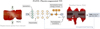 |
Fig. 3 General scheme of physics-augmented constitutive learning. From displacement fields and global reaction forces, the deformation gradient F is used to build invariant-based inputs of a constrained neural architecture. The network predicts a strain-energy density W(F), from which the first Piola–Kirchhoff stress |

5.2 Structures
The numerical capacity to solve FE problems has increased dramatically over the past decades, enabling the treatment of ever larger and more detailed models. At the same time, engineers and researchers have continuously expanded the scope of structural mechanics problems to include multiphysics couplings, multiscale effects, stochastic variability, and highly parameterized designs. This growth in ambition has revealed the limitations of classical approaches and motivated the development of new paradigms.
While the foundations of the FE method are conceptually simple, advanced basis functions and model reduction techniques—such as proper orthogonal decomposition (POD) and the proper generalized decomposition (PGD) [149]—have been introduced to reduce dimensionality and accelerate computations [150]. These methods rely on linear combinations of basis functions, and their natural extension to more expressive, nonlinear representations has brought neural networks and other machine learning architectures into the spotlight. In this context, data-driven surrogates are increasingly integrated into simulation workflows to approximate high-dimensional solution manifolds and capture nonlinear interactions more efficiently.
Yet, even with these methodological advances, the complexity of real structures and operating conditions often exceeds what purely physics-based models can faithfully represent. This gap has led to the emergence of the DT concept, which is now being enriched with data streams to create hybrid twins [74]. These hybrids combine the robustness and interpretability of nominal FE models with data-driven corrections learned from experiments or sensor feedback, thereby enabling predictive, real-time, and trustworthy simulations. This convergence between computational mechanics and data science is reshaping structural analysis, moving from purely numerical replicas toward adaptive, learning-based digital counterparts.
5.2.1 Neural solvers: PINN, GNNs, and neural operators
While the FE method remains the cornerstone of structural mechanics, nonlinear and large-scale simulations can still be computationally prohibitive. Neural networks have emerged as alternative solvers capable of approximating PDE solutions directly. Among these, PINNs and GNNs have attracted particular attention.
As introduced earlier, PINNs embed the governing equations of a physical system into the training loss of a neural network [55]. The residual of the PDE, together with boundary and initial conditions, is minimized across collocation points. Automatic differentiation allows gradients to be computed efficiently, making the method straightforward to implement in libraries such as TensorFlow or PyTorch [151]. This approach bypasses mesh discretization, offering flexibility for high-dimensional and multiphysics problems. However, convergence difficulties, sensitivity to loss term balancing, and inefficiency in highly stiff problems are well-documented [152, 153]. Research directions include domain decomposition, adaptive sampling strategies, and integration with operator-learning frameworks [146, 154].
In contrast, and again in continuity with the previous methodological discussion, GNNs treat the computational domain as a graph, where vertices represent discretization points (nodes) and edges represent FE connectivity [51]. Local states are updated by aggregating information from neighbors, mimicking the assembly of stiffness matrices in FE methods [155]. This locality allows GNNs to naturally handle unstructured meshes and variable topologies, making them promising for fracture, multiscale materials, and polycrystal mechanics [156, 157]. GNNs thus occupy a conceptual trade-off: unlike PINNs, they do not encode PDEs in the loss, but unlike black-box networks, they retain the spatial structure of the problem.
A complementary development is that of neural operators, such as the Fourier neural operator (FNO) [158] and DeepONet [56]. These learn mappings between function spaces rather than pointwise solutions, enabling mesh-independent generalization and efficient parametric PDE solving [159, 160]. Recent advances include physics-constrained operators [161] and extensions to unstructured meshes [162]. Compared with PINN, which learns one solution at a time, operator networks can generalize across entire families of problems.
Together, PINN, GNNs, and neural operators represent a new paradigm of neural solvers that extend beyond classical regression surrogates. Open research directions include improving training stability, ensuring error certification, and hybridizing with traditional solvers to leverage the best of both physics-based and data-driven paradigms. Other authors use neural networks to get a good first guess and apply Newton’s method efficiently, as in [163, 164], or a generative technique to predict solutions.
5.2.2 Homogenization and multiscale methods
Multiscale by nature when dealing with complex, architecturally structured materials, numerous methods have been developed to handle this imbrication of scales. Among them, FE2 [165] relates, for each Gauss point of a structural computation, the local stress to the local strain state history by the evaluation of a numerical unit cell problem. The main drawback is the huge memory needed to store the different histories related to the different local loading paths. Neural networks have been used to construct surrogate models of unit cell responses, thereby reducing both the storage of local histories and the repeated computational cost of solving microscopic boundary value problems.
The approach was first applied to hyperelasticity in [166] and later extended to path-dependent materials through the introduction of internal state representations [167]. In these computational studies, the full set of local state fields is accessible, unlike in experimental settings, where internal variables cannot be directly observed. Since then, numerous contributions have advanced this work [168–173].
This work on learning homogenized representations for constitutive laws shares many developments with Section 5.1.2. The main difference is the data. While for homogenization, it is possible to simulate a large number of configurations and states (including internal variables), experimental data are mainly reduced to a small number (sometimes noisy) of observable quantities. This is the reason why constitutive learning has been mainly developed in the context of homogenization.
Beyond accelerating FE2 computations, neural surrogates are also increasingly applied to the inverse design of composites and architected materials, directly tailoring microstructure to target macroscopic properties [174].
5.3 Data-driven engineering design
Data-driven approaches are impacting material and structural design, creating a continuum of methodologies that merge rapid prediction, adaptive search, and generative creativity [175]. At their foundation, surrogate models learn from high-fidelity simulations or experimental data to provide fast and reasonably accurate predictions of structural performance, replacing or complementing costly FE analyses [176] (see Fig. 4). Such models enable broad exploration of design spaces, including probabilistic assessments and sensitivity studies, at a fraction of the computational cost. Building upon this predictive capability, adaptive optimization strategies such as Bayesian optimization iteratively refine the search process by exploiting the surrogate’s knowledge and exploring uncertain regions. This reduces and accelerates the number of evaluations required to locate optimal solutions, making previously intractable design problems computationally feasible [177, 178]. Reinforcement learning extends adaptivity further by treating design as a sequential decision-making process, enabling automated exploration of design modifications guided by performance-based rewards. This paradigm is particularly relevant for complex, multi-stage problems such as topology optimization, metamaterial configuration, or adaptive structural systems [179]. At the generative end of the spectrum, deep generative models capture the underlying structure–property relationships, allowing the direct synthesis of high-performance designs without iterative trial-and-error. These include approaches from paired forward/inverse networks for targeted microstructure generation [180, 181] to VAE, GAN, and diffusion models that learn low-dimensional design representations, explore the manifold of feasible solutions, and generate novel candidates conditioned on desired performance or geometric constraints [24, 25, 182]. Across this spectrum, common themes emerge: the drive to accelerate design cycles, the need to navigate vast and complex design spaces efficiently, and the importance of embedding physical constraints to ensure feasibility and reliability. As these predictive, adaptive, and generative elements mature and integrate, they promise to redefine design workflows, enabling more innovative, efficient, and reliable engineering solutions.
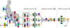 |
Fig. 4 Message-passing mechanism in graph neural networks for mesh-based learning. Operating directly on discretized geometries, such architectures provide a powerful framework for surrogate modeling, rapid design iteration (here applied for plane seats), and data-driven engineering design. Extracted from [176]. |
5.4 Structural health monitoring and digital twins
Structural health monitoring (SHM) aims to assess the integrity of structures throughout their service life by using sensor data, physical models, and data analytics to detect damage, degradation, or evolving risks. While SHM has been established for decades, the recent integration with DT concepts has profoundly changed the landscape. A DT can be seen as a continuously updated virtual replica of a physical asset, fed by real-time data and enriched with computational models, enabling not only condition monitoring but also predictive diagnostics and proactive maintenance [183].
In structural mechanics, a common strategy is to begin with a physics-based FE model of the intact structure and then augment it with sensor data to represent local stiffness reduction or other damage effects. This hybrid model can predict the current state of a structure (e.g., remaining load capacity) by combining the nominal undamaged FE model with learned, site-specific corrections, while still enforcing equilibrium and compatibility. Because the physics-based core ensures global consistency, relatively little data are required to pinpoint damage, and the resulting model generalizes naturally to unseen load cases without retraining [184, 185]. For very large structures with many subcomponents, a global physics model may ignore fine-scale details for tractability, but a data-driven augmentation can statistically account for these neglected effects, striking a balance between computational feasibility and predictive fidelity.
From an architectural perspective, DT-based SHM systems are typically organized around three pillars: (i) multi-source sensing and IoT data acquisition, (ii) hybrid simulation models that combine reduced-order FE with machine learning surrogates, and (iii) decision-support layers providing visualization, anomaly detection, and predictive maintenance planning. Reviews emphasize that this integration improves accuracy and resilience for applications ranging from bridges and wind turbines to aircraft and rail systems [183]. Hybrid approaches—where physics-based models are coupled with ML-based corrections—address key limitations of purely data-driven models by embedding physical credibility, reducing data hunger, and improving extrapolation capabilities [107,186].
Promising applications already exist. In wind energy, hybrid twins are being explored to control operating conditions in real time, ensuring reliable and optimal working loads [187]. In aerospace and civil infrastructure, DTs are deployed for fatigue prognosis, corrosion monitoring, and post-event damage assessment, leveraging probabilistic updating and Bayesian inference to handle uncertainty.
5.5 Future directions
Data-driven solid and structural mechanics has advanced rapidly, with compelling demonstrations that neural networks can learn complex, history-dependent constitutive laws; hybrid models can surpass purely empirical or purely physics-based approaches; and AI can assist in generating innovative designs and optimizing structures. These advances have been enabled by progress in high-fidelity data acquisition, scalable training algorithms, and integration of physical constraints into learning. Many building blocks are now in place, yet the field remains in an early stage of maturity, with substantial opportunities for methodological refinement, broader applicability, and deeper integration into engineering practice. This section reviews the principal limitations and outlines promising research directions. The design of ML models should also be an opportunity to formalize a number of implicit professional rules that make a good engineer.
The current landscape of data-driven solid and structural mechanics faces several interrelated challenges. Large, diverse, and high-quality datasets remain scarce, with most available data concentrated in narrow operating regimes or specific loading conditions. As a result, models trained under such constraints often display poor generalization, brittleness, and systematic bias. Similar concerns about data efficiency and transferability have been raised in the broader materials community [188]. This issue is compounded by the high cost and complexity of producing multiscale, multiphysics datasets that capture complete loading histories. Even when trained with embedded physical knowledge, predictive accuracy outside the training domain is unreliable, as subtle violations of underlying assumptions, such as changes in boundary conditions, geometry, or material microstructure, can cause significant errors. Furthermore, most current models provide only deterministic point estimates without quantifying uncertainty, leaving them sensitive to noise, outliers, and distribution shifts; the absence of standardized benchmarks reduces adoption [189]. This echoes the call for rigorous uncertainty quantification and reproducibility in materials informatics [190]. Finally, integrating machine learning surrogates into industrial FE workflows remains technically demanding, requiring robust interfacing, code portability, and rigorous verification procedures [186], with real-time deployment still a rare achievement.
Several research opportunities emerge:
Active data acquisition: Employ active learning to strategically select experiments or simulations where predictive uncertainty is highest, maximizing information gain per cost. Combine with generative data augmentation (e.g., GAN [191] and diffusion models [153]) and transfer learning to adapt models to new materials and loading scenarios.
Uncertainty quantification: Expand the use of Bayesian neural networks, deep ensembles, and stochastic surrogates. Standardized benchmarks and a posteriori error indicators could enable more rigorous model assessment and certification [154].
Advanced AI architectures: Further explore GNNs for arbitrary topologies, neural operators for parametric PDE solutions, and continuous-time recurrent models for history-dependent behavior. ML-based model order reduction could enable high-fidelity, real-time predictions in DTs.
New regimes: Extend current frameworks to fracture, fatigue, multiphysics coupling, phase transformations, and extreme event prediction. Addressing these domains will require both richer data and better integration with mechanistic models.
Emerging paradigms: Leverage foundation models and large language models (LLMs) [192] for automated code generation, model exploration, and multi-modal integration of text, images, and simulations [193–195]. Such tools could accelerate the full loop from data acquisition to validated deployment [196].
Open data and codes: Establish community-driven FAIR repositories, shared benchmarks, and standardized protocols. This would promote reproducibility, enable large-scale comparative studies, and lower the barrier for industrial adoption.
In certain domains such as living systems, recycled materials, and cultural heritage, predictive modeling is complicated by extreme inter-specimen variability arising from biological heterogeneity, uncontrolled prior histories, complex degradation mechanisms, or one-of-a-kind manufacturing processes. Data are typically scarce, heterogeneous in format, and sometimes only partially measurable, limiting the applicability of conventional large-scale training paradigms. Addressing these cases will require targeted strategies, including transfer learning from better-documented analogs, incorporation of finely tuned physics-based priors that reflect the specific constraints of the material class, probabilistic modeling to represent intrinsic variability, and hybrid experimental-numerical data augmentation to enrich the effective training set without violating physical plausibility.
The field is converging toward a physics-data fusion paradigm, where mechanistic knowledge constrains and informs learning-based components to achieve accuracy, efficiency, robustness, and explainability. Realizing this vision will depend on open resources, rigorous validation frameworks, and seamless integration into established engineering workflows [196].
6 Data-driven manufacturing processes
Manufacturing processes usually involve multiple physics and scales and apply to a large variety of materials. In what follows, we will consider polymers and reinforced polymers, composites, and metals.
During the manufacturing process, these materials experience very large multiphysics transformations, many times involving a sequence of individual operations, that gradually transform the raw material into a formed part with its own shape, topology, internal microstructure, and the associated properties and performances. Nowadays, performances go beyond the simple mechanical ones. Components are in turn assembled in larger structural systems, making use of appropriate assembling operations.
Thus, manufacturing processes represent a series of combinatorial choices involving, e.g., material, process, and assembling as well as the elementary operations sequencing that, in turn, has its own combinatorial set of possibilities.
6.1 Numerical technologies
A holistic approach to manufacturing processes needs at least four main numerical technologies:
Collecting existing knowledge. Identifying the most valuable multiphysics and multiscale model describing the material and process couple, as well as the numerical technology enabling its efficient solution (e.g., model order reduction and surrogates). Here, the physics-based knowledge should be augmented with all the existing expert domain knowledge as well as all the constraints applying to the material and processing.
Observing. Identifying the data to be collected on the material all along its transformation and on the processing machines. The knowledge of the first-order model (previous item) serves to identify the type of data enabling the highest observability of both the material transformation and processing conditions. As previously mentioned, smart or useful data should respond to four questions: which data, at which scale, where, and when are they collected? In general, manufacturing processes manipulate a large range of data typologies, among them numeric or categorical data, images, curves, time series, etc.
-
Describing. As previously discussed, the collected data are sometimes too rich, and sometimes it contains too many linear and nonlinear correlations. Even if technologies to proceed directly from the acquired data exist, sometimes, extracting descriptors or transforming the data to obtain more compact representations represents valuable routes to facilitate model training in machine learning technologies.
The three most common approaches consist of the following:
The descriptor coincides with the collected data itself. This is the case, for example, when diagnosis, prognosis, or decision-making follows directly from the collected data without any manipulation applied to it.
Data transformation looks for an automatic extraction of features that the data contains, enabling a complexity reduction. This is the case when applying the Fourier transform on a time signal, a wavelet transform on an image, or TDA (topological data analysis) to images, curves, or time series [16].
Statistical descriptors operate on the collected data to provide some quantities that are expected to be the ones on which the involved physics depends, such as, for instance, phase volume fractions, polydispersity of grains, pair-correlation to describe entities’ distribution, etc. [22].
-
Modeling. Models are expected to provide an output (e.g., field and quantity of interest) from the input appropriately described as just discussed. The outcome of a model could be a label, as supervised classification performs, or continuous variables, in the case of regression. As described before, there is a panoply of choices, depending on the typology and volume of the manipulated data.
Two variants of data-driven modeling can be differentiated:
Fully data-driven, in which the model is learned from the available data by using an appropriate machine learning technology;
Informed or augmented, that as previously described, the existing knowledge (first item above), including physics-based models, expert domain knowledge, or constraints, is included in the learning process.
In what follows, the different choices concerning observation, description, and modeling will be applied to three major types of materials: (i) polymers and reinforced polymers; (ii) composites; and (iii) metals.
6.2 Polymers and reinforced polymers
Polymers are composed of macromolecules, entangled or in solution with a solvent. Rheology is a complex matter because the macroscopic behavior depends on a number of variables describing the molecular conformation, such as, for instance, orientation and extension of the end-to-end vector or of the different segments assumed to represent the macromolecule. Thus, an adequate integration of that molecular level into the macroscopic behavior is needed, together with a model governing the evolution of the molecular conformation (e.g., end-to-end vector orientation and extension) induced by the flow.
An additional difficulty comes from the highly dimensional character of the molecular description, which can imply tens or hundreds of conformational coordinates involved in the conformation time evolution equation, at the origin of the curse of dimensionality that the solution of those models implies. The interested reader can refer to [197] and [198] for a deep introduction to complex fluids modeling.
When parts made from polymers (plastics) do not meet the targeted performances, they can be reinforced by the use of short reinforcement, ranging from the nanoscale (e.g., CNTs, nanofibers) to the macroscale (millimeter or centimeter fibers). These charges offer both mechanical and functional properties, both of them depending on their final distribution, which in turn is induced by the flow during processing.
6.2.1 Reactive extrusion
Reactive extrusion is a complex but widely employed processing technology where different physics meet: complex fluid flow, reactant mixing, chemical reactions with their associated thermal couplings, heat transfer, etc., a fact that limits the existence of accurate high-fidelity physics-based models. Today, only simplified models are available, being, in most cases, inefficient to predict all the quantities involved in the process: advancement of reaction, temperature, pressure distribution, etc.
Because of such a difficulty, two different approaches were considered in [199] and [200].
In [199], a series of processes and input material parameters were identified, as well as the properties of the resulting material. Then, different regressions were considered for inferring properties from the input data, while determining the more sensitive input parameter to each measured property of interest associated with the extruded material.
On the other side, in [200], an augmented approach was considered. First, a simplified physics-based model, adequately calibrated, was employed, and their predictions were compared with the experimental measures. Then, the measure versus prediction gap was used to learn the model of the gap, within the augmented or hybrid rationale. Thus, the enriched simplified model was able to accurately predict the process.
6.2.2 Extrusion
Another important issue when performing extrusion is the prediction of the final extruded profile that deviates from that of the die because of the die-swelling phenomenon characteristic of non-Newtonian fluid behaviors (normal stress differences). Obtaining the right extruded geometry requires designing an appropriate die, such that after swelling, the extruded geometry corresponds to the target. The limitations in the numerical analysis of non-Newtonian fluid flows limit the use of numerical simulation for designing the right die to obtain the right profile.
It is in these circumstances that machine learning can represent an appealing route for such an optimization. In [201], the authors used an autoencoder to extract the latent representation of the die profile. Another autoencoder reduced at its turn the measured final profile related to each die geometry. Then a multilayer perceptron was used to connect both latent representations, the one of the die profiles and the one of the resulting extruded profiles. Thus, as soon as a die is considered, the die encoder applies, and then the MLP connects with the reduced extruded profile that, after decoding, provides the final extruded geometry. On this basis, design and optimization can proceed in a very efficient manner.
The same procedure could be employed not to predict the extruded profile but to predict the correction to apply to the numerical simulation-based prediction within the hybrid or augmented rationale.
6.2.3 Distortion of injected parts
Plastic injection is another widely employed processing technology that, despite its longevity, continues to elude springback predictability. Part distortion results from residual stresses induced during the solidification process, which could be exacerbated by the anisotropy associated with the use of reinforced polymers.
A surrogate providing the distortion field as a function of the different material and process parameters can be easily elaborated upon. In order to avoid the fact of manipulating too rich representations, one possibility consists of performing a linear (PCA, for instance) or nonlinear (e.g., autoencoder) reduction of the distortion fields and then constructing a regression between the material and process parameters and the reduced (latent) parameters describing the distortion.
A similar, but maybe simpler procedure can be employed to connect material and process parameters with a goal-oriented quantity of interest, quantifying the distortion.
6.2.4 Short fiber composites
When using short fibers suspended in a polymer matrix, the rheology depends on the concentration and orientation of the fibers, with the fiber orientation distribution induced by the flow [197].
Macroscopic behaviors are usually derived from fine-scale micro-mechanical modeling; however, the scale-up enabling a closed constitutive equation needs the introduction of a series of hypotheses and assumptions whose validity can be compromised in many situations.
In general, the observed flow and orientation distribution deviate significantly from the one predicted by state-of-the-art models, even when considering the most sophisticated ones.
It is then in these circumstances that the use of data-driven approaches can be a valuable option, not to derive models from scratch but for enriching the predictions by adding to the state-of-the-art physics-based model a data-driven model expected to represent the prediction to the data gap.
In [202], the orientation model was improved beyond the limits of state-of-the-art models.
When considering rheology, our recent works aim at discovering the extra descriptors (other than the second or fourth order orientation tensors) enabling the description of the measured rheology, while including in the learning procedure the fact that second and fourth order tensors should be considered as suggested by micro-mechanical models [197].
6.2.5 3D printing
3D printing addresses some of the previously mentioned difficulties, including the geometry of the deposited extruded filament on the substrate already printed, which leads to the accumulation of inaccuracies, and the dynamic evolution of part distortion related to the progressive solidification of the deposited layers.
Here, machine learning is used for many purposes, among them: (i) ensuring the geometrical conformity by actively controlling the process; (ii) avoiding defects related to porosity generation; (iii) defining optimal deposition trajectories; (iv) optimizing the resulting microstructure; and (v) enabling a gradient of properties.
6.3 Composites
6.3.1 Sheet molding compound—SMC
In general, short fiber composites are elaborated from both extrusion and injection, and as just discussed, the main objective is an accurate prediction of the final fiber orientation and distribution because properties and performances, beyond the mechanical ones, are strongly impacted by the fiber distribution and orientation.
SMC consists of a compression molding process. The so-called preform, consisting of fibers and a resin mixture, the so-called charge, is placed in the open mold, which, when closed, compresses the charge, filling the mold.
Here, the reinforcement, small patches or centimeter-length fibers, flows while orienting because of the flow velocity gradient.
Predicting the final fiber distribution and orientation is of major interest for evaluating the final material properties and part performances. The high fiber concentration in SMC with respect to the one usually considered in reinforced polymer injection or extrusion challenges state-of-the-art orientation models, the last derived in general for dilute or semi-dilute concentration regimes.
Here again, machine learning could help to increase predictability by learning the orientation descriptors and the dynamical system governing its evolution to enrich the usual ones, whose validity is restricted to small fiber interactions and quasi-Newtonian fluid behavior.
Another crucial aspect in SMC processes consists of determining the optimal shape and location of the preform in such a way that after its compression its shape becomes the one of the considered part, that is, the flow front and the end of the compression stage reach the mold boundary simultaneously, a situation that ensures process optimality (minimum compression force) and enables better fiber orientation predictability.
In [203], authors considered a high-fidelity filling process simulator. The flow front was parametrically described by using a rich enough spline representation, defined by a number of control points. For any final target shape, the simulation was performed by decompressing instead of compressing until reaching the initial stage that represents the initial charge shape, also described by a spline with the same number of control points. Now, a model expressed by a neural network can learn to infer the initial charge shape depending on the targeted final shape.
6.3.2 Resin transfer molding—RTM
RTM consists of impregnating a porous preform with a resin that, after curing (thermosets) or polymerizing (thermoplastics), will constitute the composite structure. Many reinforcement architectures exist that condition permeability.
The main usual defect during the filling process is that air remains trapped in between flow fronts that meet, creating unfilled regions. Another issue comes from the fact that the flow velocity inside the yarns and in between the yarns is different, and if that difference is important, porosity occurs. Infusion is based on the same principle, but instead of a rigid mold, it processes from a transparent bag that allows for computerized vision.
When operating on images, convolutional neural networks can process them and, from them, anticipate defects or porosity, enabling performant control procedures to ensure good quality filling.
When molding very large structures, the accumulative effects of heterogeneities, uncertainties, and variabilities produce a noticeable deviation between the predicted flow front evolution and the one observed from images or from a sensor network deployed in the mold. In that case, predicting the whole filling process becomes uncertain, and unexpected defects can occur.
To keep predictability all along the molding, a hybrid rationale can be applied in order to ensure the agreement between the flow front prediction and the observation by modeling the noticed gap as described in [204].
In all cases, the uncertainty on the model and process parameters must be incorporated into the predictions by formulating the problems in a probabilistic setting, where, more than a deterministic surrogate, a parametric confidence interval is predicted.
6.3.3 Automated tape placement—ATP
ATP enables the manufacturing of large and complex structures, thereby challenging more conventional manufacturing processes.
The process, as well as the aspects concerning its thermo-mechanical modeling and simulation, is described in numerous references [205].
The main difficulties concern the strong multiphysics coupling involving heating, heat transfer, roughness evolution, thermo-mechanical coupling (melting and solidification), field localization, and fast dynamics, which challenge models and simulation technologies.
ATP involves 3D effects present in the almost 2D geometries (tapes with the thickness orders of magnitude smaller than the other representative dimensions).
Model order reduction techniques, based on parametric surrogates, were successfully applied for simulating the different components of the whole process [205]. These surrogates employed regularized linear polynomial regressions in tandem with in-plane-out-of-plane separated representations that enabled considering 3D effects in the almost 2D tape geometries.
A major challenge concerns the multiple scales induced by roughness or by the heterogeneity of the fibers and pore distribution and their impact on the thermo-mechanical properties.
ATP, as just described, is based on the consolidation of a composite tape on the one already deposited. For that, heat and pressure are applied to ensure the highest degree of intimate contact enabling molecules to reptate across the interface to reach the bulk characteristic properties.
However, tape surfaces exhibit an inherent roughness that strongly impacts the time evolution of the degree of intimate contact. The asperities characterizing the roughness are squeezed and flow; however, such a squeeze flow not only depends on the thermo-dependent rheology of the polymer or the composite and the applied pressure but also on the roughness itself.
Usually, to infer the process window, that is, the adequate heat and pressure applied to obtain the targeted DIC for a particular roughness, the latter must be described by an adequate descriptor.
The use of the roughness profile itself as input data could be possible; however, a lot of surfaces will be needed when using such multiscale data in the learning process. To reduce the cost, the use of an adequate descriptor seems a better option.
Statistical descriptors based on the statistical analysis of the different asperities composing the rough profile are inefficient to explain the observed physics, that is, the time evolution of the degree of intimate contact. More advanced statistical descriptors were proposed in [206], where micro- and macro-curvature played an important role in the properties’ inference.
Some works made use of more sophisticated descriptors like the fractal dimension, the Hurst index related to anomalous diffusion generating random walks describing the roughness, wavelet representations, and so on.
Possibly, the best descriptor that enabled surface classification and degree of intimate contact estimation consisted of using TDA (topological data analysis) that extracted the profile topology features [19].
However, the choice of the descriptor without taking into account the goal in its use entails a certain level of risk that manifests in poor predictions of the physics under scrutiny, for example, the time evolution of the DIC.
Certainly, the best option consists in extracting (discovering) the descriptor associated with the roughness that enables predicting the physics under consideration. RRAE introduced at the beginning of the present paper enables enforcing that the first latent modes must represent at best the physics that is expected, depending on the surface roughness. This approach constitutes a new paradigm in physics, where goal-oriented descriptors are extracted simultaneously with model learning.
6.3.4 Homogenization and localization
Sometimes one is interested in predicting fields or Quantities of Interest (QoI), which in general are related to, for example, localized hot spots and temperature gradients in extremely heterogeneous media that usually involve composite materials.
These materials exhibit several phases (fibers, resin, and pores) that are distributed differently throughout the tape. Thus, for a given phase distribution extracted from an image, one would like to infer the temperature distribution, for instance (or the flow during impregnation, or stresses during curing, etc.); however, meshing the domain and performing a FE simulation, for instance, becomes computationally demanding, compromising real-time control.
Predicting in real-time those fields for a given microstructure is not an easy task, despite its high interest.
In [207], authors used adapted neural architectures, U-Net with co-attention mechanisms, to operate on the microstructure images that were completed with some derived fields (time-of-flight) to infer in real-time the temperature field in any given microstructure, as illustrated in Figure 5. A similar approach could be considered for evaluating the intra-yarn flows during resin impregnation.
When looking for effective properties (homogenization), training such a network seems too computationally demanding. Again, a possibility could consist of providing the microstructures to a convolutional RRAE encoder while enforcing the first latent modes to infer the effective properties.
 |
Fig. 5 Inferring the temperature field for a given composite microstructure. The model is a U-net architecture with a two-branch encoder, attention mechanisms, and fusion modules. Extracted from [207]. |
6.4 Metals
6.4.1 Additive manufacturing
In the case of additive manufacturing, the problem is quite close to the one considered in 3D printing. Artificial intelligence and machine learning were widely considered for predicting defects and evaluating the process window, enabling its minimization. Such a model is of critical significance in process control [208].
6.4.2 Casting
In the domain of casting, many physical phenomena coexist. The temperature field is governed by the heat equation, and the associated temperature field that depends on a series of material and process parameters can be expressed from quite simple and accurate regressions.
The situation is radically different when considering porosity nucleation and pore growth, where both mechanisms exhibit locality, that is, both depend on the local state and local thermo-mechanical history, making it difficult to use the usual regressions as discussed in [209], where the authors proposed a local model able to infer the porosity appearance.
Concerning the evaluation of global fields, such as the temperature field, noticeable deviations appear between the prediction of high-fidelity physics-based models and the temperature provided by a series of thermocouples. In [210], the authors proposed, within an augmented learning framework, completing the gap measured at the thermocouples’ locations across the entire domain by using a reduced basis provided by the physics-based model. Then, from the gap defined everywhere, a surrogate was learned to infer it from the process and material parameters used to construct the physics-based model surrogate. When combined, these two ingredients define a highly accurate casting hybrid twin, enabling extremely fast inference while requiring only a limited amount of data [210].
6.4.3 Stamping
Following the same rationale, a stamp hybrid twin was considered in [186]. A nominal stamp was simulated for different materials and processing conditions, and the associated thermo-mechanical fields (e.g., plastic strain and deformation) were expressed through linear or nonlinear regressions based on those parameters. Plastic deformation exhibits a high degree of localization, and in that case, it was proved that performing clustering and elaborating a surrogate in each cluster provided excellent results as soon as one was able to infer the cluster to be considered from the provided parameters (classification).
When a gap between the predictions and the measurements is noticed, the gap data are extended to the whole domain to define the gap field, and then that gap field is regressed with respect to the model parameters to define the so-called stamp hybrid twin.
6.4.4 Riveting
Simulating riveting is computationally demanding because, first, a rich enough thermo-elasto-visco-plastic model must be selected and employed after calibration. Second, the finite element meshing and simulation are very time-consuming. After simulating the whole 3D process, different quantities are evaluated to quantify the riveting quality in order to determine the process window related to the choice of the process parameters.
In [211], the authors assumed that quality factors depend on the material and process, but the latter, in a certain manner, are encapsulated in the measurable force-displacement curve that the riveting machine provides. A model was learned to connect that curve to the quality indicators as illustrated in Figure 6, exhibiting excellent performance.
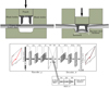 |
Fig. 6 Inferring riveting quality parameters from the processing force-displacement curve. The machine learning model is composed of a convolutional autoencoder (top) and a multilayer perceptron acting in the latent space (bottom). Reproduced from [211]. |
6.4.5 Welding, induction, and other processes
Welding represents another widely used assembling process, where again predictions and measurements can exhibit a noticeable gap, in particular when the welding device loses its effectiveness due to aging. Beyond calibration, model predictions must be enriched (or corrected) in order to improve accuracy and enable the identification of the optimal process window. Spot welding sequencing is another hot topic, because of the associated combinatorial explosion, where reinforcement learning could help to manage that difficulty.
There are many processes in which physics-based models are not accurate enough, as it is the case considering electromagnetic induction for improving the surface properties of forged parts. Here, fully data-driven or hybrid models [212, 213] are appealing approaches for attaining the degree of predictability enabling process optimization.
7 Data-driven fluid mechanics
The recent rise in high-fidelity numerical simulations (DNS, LES) and high-resolution experimental diagnostics (PIV, tomographic PIV, and time-resolved sensors) has ushered fluid mechanics into the age of data [214, 215]. In this context, the convergence between computational fluid dynamics (CFD) and machine learning (ML) opens exciting new opportunities [216], including (i) discovery of coherent structures and reduced latent representations, (ii) fast emulation and forecasting of complex flows, (iii) data-assisted discovery of closure or constitutive models, (iv) acceleration or improvement of existing solvers through learned components, and (v) super-resolution and data assimilation. The following subsections review these directions and highlight recent advances as well as current challenges.
7.1 Unsupervised learning and flow-structure discovery
Modal decomposition techniques have long been central to fluid mechanics for identifying dominant flow structures. In the early stages of data-driven analysis, most studies involved the application of basic data science techniques to canonical fluid flow problems to analyze and model flow physics. Such approaches often leveraged linear decomposition techniques, such as POD and DMD, which extract coherent motions and their associated temporal dynamics from flow data. A comprehensive overview of DMD and its extensions can be found in [217].
However, the governing equations of fluid dynamics are intrinsically nonlinear, leading to the rapid breakups of linearized models after a short time horizon. With the advent of modern ML, nonlinear manifold learning has complemented linear model methods. AE, VAE, and kPCA can embed complex flow fields into low-dimensional latent spaces, capturing nonlinear correlations. Early examples date back to the beginning of the 2000s [218] with applications to wall shear stress reconstruction in a low-Reynolds number turbulent channel flow. In [219], AEs were shown to find accurate low-dimensional representations of flow dynamics behind a circular cylinder. Recently, Fukagata et al. have used AE to find low-dimensional manifold representations of chaotic flow fields [220] and to model their dynamics in such a reduced space. AEs pretrained on diverse flows have been used recently for vortex identification [221], appealing to the arbitrary definition and empirical thresholds required by physics-based vortex identification criteria. The model is first pretrained on diverse datasets using a self-supervised strategy, and then it is fine-tuned on specific cases using limited labeled data. The works of [222, 223] used convolutional neural networks in conjunction with nonlinear sensitivity analysis, namely, the Shapley additive explanation values (SHAP) [224], to extract coherent structures in wall-bounded turbulent flows (see [225] for a thorough definition of coherent structures) and relate them to momentum and energy transfers between the flow and the wall.
Due to the complexity of fluid flows, several dynamical processes may coexist in the same field. In such cases, it is of both scientific and practical relevance (in view of modeling) to identify the dominant processes automatically by using unsupervised machine learning and, specifically, clustering algorithms. A meaningful early example is provided by the work of [226], who introduced a cluster-based reduced-order modeling algorithm (CROM) capable of generating clusters of time snapshots of a flow field based on their similarity via the popular k-means algorithm, while determining a transition probability from one cluster to another. This allows identifying the characteristics of dynamical system attractors directly from data. Saetta and Tognaccini [227] used a probabilistic clustering algorithm, namely, Gaussian model mixtures (GMM) (e.g., [228]), to automatically identify flow regions characterized by similar spatial dynamics (free streams, boundary layers, and shocks) in steady flow solutions. The GMM approach shows promise to overcome some limitations of classical physics-based flow decomposition criteria, which require the adoption of case-dependent cutoff inputs, topological information, and a final human check. On the other hand, the clustering is based on a set of engineered flow features, and the results are sensitive to feature choice.
A promising approach for dominant flow process identification based on prominent terms in the underlying governing equations has been introduced by [229]. The methodology consists of two steps. In the first step, GMMs are applied to a set of data points with coordinates corresponding to the terms in the underlying governing equations. Then, sparse PCA [230] is used to select the hypothesis that better represents the cluster dynamics, i.e., the terms with the largest variance in the cluster. Their methodology, called the dominant balance approach, was able to successfully delineate dominant balance physics in diverse dynamical systems, including time-averaged turbulent flow fields. However, its success largely depends on SPCA and its associated tunable hyperparameter, i.e., the magnitude of the least absolute shrinkage and selection operator (LASSO) [231] used to determine the SPCA components. Kaiser et al. [232] introduced an optimality measure for the identification of dominant balance processes from data. The measure can be applied to evaluate different choices of both the clustering and hypothesis selection methods and demonstrates its effectiveness for problems including ocean dynamics and turbulent boundary layers.
Collectively, the above-mentioned approaches constitute novel and promising tools for extracting relevant flow features and processes from data and provide low-dimensional representations of complex dynamics for further prediction or control tasks.
7.2 ML-based flow emulation and forecasting
Fluid dynamics problems are inherently computationally intensive due to the large number of degrees of freedom required to capture the relevant flow scales and the flow nonlinearities. As a consequence, ML has been widely employed to emulate the dynamics of fluid flows, thus replacing costly traditional numerical solvers (based on finite volume, finite difference, or finite element methods) for fast prediction of global performance parameters, local distributions of quantities of interest, or full flow fields. The emulators are key for accelerating multi-query problems, such as design optimization, control, uncertainty quantification, and data assimilation, where a large number of calls to the numerical solvers are needed, rendering brute-force calls to flow simulators unfeasible. In this setting, it is possible to distinguish three distinct families. The first family includes parametric surrogates, which aim at reproducing the system response, represented by any field  (with x being the spatial location and t being the time), as a function of a vector of P input quantities
  , such as geometry-determining variables, boundary conditions (operating conditions), or fluid properties, for a parametrized class of flows. Most surrogates address steady-state problems, for which only the dependency of the steady-state fields is sought in terms of the problem input parameters:
  . The second family corresponds to emulating the time dynamics of the problem for a given choice of the parameters
  , and eventually forecasting the system behavior beyond the observed time horizon. The modeling target is then the generic field
  . The third one is a combination of the previous ones and consists of modeling the time dynamics over a set of input parameters, including flow conditions and/or geometries. The modeling strategies used to build the emulators tend to differ depending on the target surrogate modeling problem. Note, however, that the boundaries across the above-mentioned applications can be quite blurry, and some approaches can serve for several modeling tasks.
7.2.1 Surrogate models for parametric problems
In the case of parametric surrogates, the modeling target is most often a scalar quantity  or a field variable
  representative of the steady-state flow behavior. This kind of modeling is generally required for efficiently exploring design spaces in view of optimizing the system performance or for performing uncertainty quantification. Gaussian processes [233, 234], sparse polynomial projections [235, 236], or deep-learning approaches have been used for such purposes. For scalar modeling targets, the main limitation is generally represented by the curse of dimensionality problem when the number of parameters grows (e.g., [237]). The former can be addressed by coupling surrogate models with dimensionality reduction strategies based on active subspaces [238], PCA projections [239], AE [240], or implicit neural representations [241]. For field variables, the same techniques can be used to find a reduced representation of the target fields first and then model the dependency of the reduced latent variables on the parameters μ. A critical bottleneck is represented by the robust handling of variable geometries, an area where existing methods have shown significant limitations [242, 243]. The variation of boundaries in the physical domain poses a major challenge when building ML surrogate models. In fact, such models usually perform poorly on tasks that require learning functions or operators defined on mutable supports. Moreover, problems characterized by high Reynolds numbers or strong compressibility effects may exhibit thin boundary layers and high gradients, which concentrate most of the relevant information in small regions of the domain and are particularly challenging for surrogate models to learn accurately [244].
7.2.2 Emulators of reduced time dynamics
The modeling task consists of emulating the time dynamics of a fluid flow system, i.e., modeling the time evolution of the system state variables  for a given set of flow conditions
  (e.g., initial and boundary conditions). Reconstruction of flow dynamics from flow snapshots has been attempted by a number of authors, especially with the aim of real-time modeling and flow control. The techniques in use range from reduced-order models based on linear [217] or nonlinear projection methods [14, 245–247] to hybrid POD/AE or AE/Galerkin projection methods [248, 249], based on previous works such as [250]. Other kinds of deep-learning emulators have been proposed, based, for instance, on neural ordinary differential equations (NODE) [251] or recurrent neural networks, including long short-term memory (LSTM) models [252, 253]. Such approaches are generally coupled with dimensionality reduction techniques that first project the spatial fields onto a reduced latent space, where the latent variables are processed (advanced in time) and finally decoded in the initial space. Most models exhibit stability problems when applied beyond the training time horizon, quickly diverging from the target physical solution, especially for chaotic flows [254]. This problem can be in part mitigated by moving from purely data-driven training strategies to equation-driven approaches where the residuals of the underlying governing equations, the boundary conditions, or other physical constraints are used to inform the model parameters in addition to data [55, 255, 256]. When the physical constraints are handled in weak form through the addition of Lagrange multipliers to the data-driven loss function, the class of so-called physics-informed machine learning methods, including the popular PINN family, is recovered. Of interest, in the limit case when only the equation-based loss (or “residual”) is used to drive the search, physics-informed emulators can be assimilated to the family of meshless discretization methods, such as smoothed particle hydrodynamics (SPH) [257] or gas-kinetic schemes (GKS) [258]; from a machine learning perspective, residual-only PINN belongs to the class of unsupervised learning methods since no data are used to guide the search. This property is particularly attractive for fluid flow applications, for which data generation is particularly costly, and flow data samples can be extremely cumbersome, requiring the storage of large 3D and time-resolved data sets. Unfortunately, purely residual-driven training tends to be ineffective compared with classical numerical methods for fluids, namely for complex problems of engineering interest [259]. The latter are in fact characterized by high irregularity and steep gradients, leading to great sensitivity of the results to the number and location of collocation points used to estimate the residual and to convergence and stability issues, particularly for advection-dominated flows [260]. Remedies to such drawbacks represent a very active field of research.
7.2.3 Neural operators
Most of the reduced-order models or machine-learning emulators cited above are targeted to reproduce a single flow configuration or a narrow flow class (e.g., 2D airfoils, a family of car shapes, etc.) defined over some parametric space (e.g., the geometry or operating conditions) for digital twinning [261] or data assimilation [262] purposes. Recently, thanks to the increased availability of larger datasets, considerable interest has been developed in general ML emulators, allowing the exploration of large parametric spaces, with the aim of potentially replacing classical general-purpose fluid dynamics solvers over a variety of configurations. This has fostered the development of parametrized emulators, or so-called neural operators, which include now popular methods such as the FNO [158] and DeepONet [263]. The role of neural operators is to learn mappings between function spaces instead of individual solutions. For geometry-independent problems, they have shown good generalization across boundary conditions. For example, FNO architectures have achieved accurate predictions of turbulent channel flows up to  [264]. In geophysical applications, large-scale neural operators, such as FourCastNet [265] and GraphCast [266], have demonstrated five orders of magnitude faster weather forecasting compared with numerical weather prediction systems. Such models, pre-trained on very large datasets, belong to the class of so-called “foundation models,” and they represent a recent research pathway actively explored by several groups with a focus on families of PDEs, including governing equations for fluid flows [267–269], following major breakthroughs achieved in weather and climate sciences.
For engineering flows, however, operator learning remains challenging and costly: complex geometries, multiphysics coupling, and limited training examples hinder generalization. While most neural operators are purely data-driven, physics-informed versions have been proposed in the aim of reducing the need for data and improving generalizability. Physics-informed neural operators [270] incorporate PDE residuals into the loss function, while equivariant networks [271] explicitly encode physical symmetries. As an alternative, Wu et al. [272] have proposed the use of transformer architectures to enforce physical context via the attention mechanisms [72]. Enforcing conservation and physical constraints, handling complex geometry, scaling efficiently to 3D problems, and tackling chaotic, multiscale phenomena such as turbulence remain active research areas and keys to make machine learning methods competitive with respect to classical computational fluid dynamics.
7.3 ML-assisted model discovery
A central application of ML in fluid mechanics lies in the discovery and augmentation of closure models: turbulence, transition, roughness, rheology, or reaction-rate models for some coarse-grained version of the flow governing equations. Coarse-grained approaches are used to reduce the range of scales directly captured by the flow models, which can become extremely costly or just unfeasible in some situations, by modeling the physical scales below a defined threshold. Such an approach represents the workhorse for engineering turbulent flow modeling, where the Navier–Stokes equations are filtered (leading to so-called large eddy simulations, or LES) or averaged (leading to Reynolds-averaged Navier–Stokes (RANS) approaches). Coarse-graining generally produces unclosed terms that are traditionally modeled via a balanced mixture of physical knowledge, empiricisms, and cost-accuracy compromises, thus introducing significant cost reductions but also large uncertainties in the model’s predictive accuracy depending on the chosen model structure and the determination of the associated tunable parameters (see [273] for a review of turbulence modeling uncertainties). Data-driven turbulence modeling is now a mature research area, as reviewed in [274–276]. Neural networks have been trained to predict sub-grid stresses in LES or Reynolds stresses in RANS. Nowadays, data-driven turbulence modeling has become one of the most active research topics in computational fluid dynamics. Of note, recent ML advances in turbulence modeling have increasingly incorporated physical priors through grey- (neural-network-based with physics-informed architectures) or open-box (i.e., based on symbolic regression methods) approaches that learn corrections to a baseline turbulence model using appropriate physics-informed functional bases [277–280]. Yet, data-driven ML models often generalize poorly outside the class of flows for which they were trained, and special care must then be taken in complex flow applications, where multiple flow processes may coexist. Strategies for improving generalizability involve multi-objective training [281], model mixtures [282–285], and progressive augmentation [286]. A more complete overview of data-driven approaches for turbulence modeling can be found in the book chapter [287]. In addition to turbulence modeling, examples of data-driven model discovery can be found in rheology [288, 289], thermodynamics [290], particle flows [291], and reactive flows [292], among others.
These developments bear strong similarities with data-driven constitutive modeling in solid mechanics, discussed in Section 5, where the objective is likewise to enrich or replace partially known closure relations from data while preserving physical consistency.
7.4 ML for acceleration and enhancement of numerical solvers
Rather than replacing CFD solvers, ML can accelerate their most expensive components or improve their predictive accuracy. Recent studies have demonstrated acceleration of CFD solvers via machine learning-based initialization [293], computational speedup of incompressible flow simulations via learned surrogates for the costly Poisson equation solver [294], and fast thermophysical model evaluations for real-gas or reacting flows [295–297]. ML has been coupled with mesh adaptation techniques for initial mesh generation [298] and fast prediction of mesh node/solution relationships that can then be optimized according to prescribed criteria [299] to target refinement regions using clustering methods [300] or locally adapt the solution reconstruction order [301]. ML methods have also been used to speed up time-stepping schemes while avoiding the burden of solving large linear systems [302–304].
A particularly interesting line of research is represented by hybrid CFD-ML solvers, or “solver-in-the-loop” ML approaches, whereby an imperfect CFD model, affected by numerical approximation errors or modeling assumptions, is augmented with a companion ML model. The ML model can be incorporated in several ways: as an external correction applied to the model output [305], as an additive correction to the model residuals within the time stepping loop [306], or as an internal correction embedded directly into the solver’s equations [307]. The latter requires a differentiable CFD solver, since updates must be propagated through the solver before being back-propagated into the ML model. Such approaches are generally more computationally demanding than the non-intrusive emulators described in Section 7.2.1, because they involve repeated calls to the expensive direct (and sometimes adjoint) solvers. However, they typically yield greater stability over long roll-outs. In addition, Hybrid CFD-ML frameworks are also appealing from an engineering standpoint: the core solver remains physics-based and trusted, while ML components target specific, computationally intensive sub-tasks. However, their integration within legacy solvers raises challenges of numerical stability, training data representativeness, and certification.
7.5 Super-resolution and data assimilation
Super-resolution techniques aim to reconstruct high-resolution fields from coarse CFD outputs or sparse measurements. CNNs, GANs, and diffusion models have been applied to infer fine-scale turbulence structures. For example, Fukami et al. [308] used a hybrid downsampled skip-connection multi-scale network based on a CNN backbone to super-resolve 2D homogeneous turbulence and turbulent channel flows. Deng et al. [309] used super-resolution generative adversarial network (SRGAN) and enhanced-SRGAN (ESRGAN) to augment the spatial resolution of turbulent flow data. In experimental settings, ML-augmented data assimilation can reconstruct velocity and pressure fields from sparse PIV data, combining ML with Bayesian or adjoint formulations [310, 311]. Super-resolution methods are increasingly integrated into digital-twin frameworks, where coarse CFD predictions are continuously corrected using real-time sensor data [312]. An ongoing challenge is ensuring that reconstructed fields satisfy key physical constraints such as mass, momentum, and energy conservation and reproduce accurate turbulence statistics and spectra. Figure 7 illustrates the structure-preserving super-resolution technique proposed in [313]. A recent overview of these developments is provided in [314].
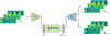 |
Fig. 7 Structure-preserving super-resolution neural architecture. First, an encoder is used to reduce the dimensionality of the problem, obtaining a set of reduced variables or latent code. Then, a structure-preserving neural network (SPNN) is trained to integrate the time evolution of the reduced variables of the system. Finally, the decoder is used to recover the data to its original dimensionality and to generate the output in a resolution that is higher than the input one. Reproduced from [313]. |
7.6 Outlook
The convergence of ML and CFD is entering a mature phase. Future directions include:
Foundation models for fluids: Present machine learning emulators are limited to narrow flow classes and need retraining whenever a new configuration is targeted. Given the high computational cost of CFD simulations, repeatedly retraining surrogate models is both time-consuming and inefficient. Transfer learning [315] and in-context learning [316] can mitigate part of this burden, but more systematic strategies for reusing information acquired from previous tasks are needed. In particular, the development of large-scale neural operators pretrained on diverse flow configurations offers a promising avenue to leverage prior knowledge and substantially reduce the amount of data required for adaptation or retraining. Achieving this vision, however, hinges on the availability of large, high-quality, and carefully curated datasets—an objective that will require a significant, coordinated effort from the community.
Multi-fidelity and active learning: Given the large amount of data required to train ML models, samples obtained from low-fidelity CFD models are typically used as the training examples. As a consequence, the ML model accuracy cannot be better than the generated data. However, pushing the boundaries of fluid flow modeling requires high-fidelity, scale-resolving simulations that, while extremely detailed, can be produced only in limited quantity due to extreme computational burden, especially for complex configurations of engineering interest. The development of models that can learn from data of different fidelities [317–320] can effectively fuse a large amount of low-fidelity information with selected, well-chosen high-fidelity samples, thereby improving the overall model quality.
Explainability and interpretability: Most machine learning methods operate as black-box function approximators. As such, they typically lack both explainability (the ability to articulate why a given prediction is produced) and interpretability (a transparent understanding of the model’s internal representations). This stands in clear contrast to classical physics-based models in fluid mechanics, which are inherently explainable and interpretable, enabling modelers to adjust parameters and interpret outputs in light of established physical principles. To help bridge this gap, symbolic approaches such as SINDy [34] and modern explainable ML techniques [321] can be combined with traditional machine learning tools, providing more transparent and physically grounded workflows.
Uncertainty quantification: providing interpretable estimates of the predictive uncertainties of ML-augmented CFD models and surrogate emulators is essential for industrial deployment, particularly in safety-critical sectors such as nuclear energy and aerospace. Yet robust uncertainty quantification remains challenging—especially for out-of-distribution predictions—because most existing techniques significantly increase training and inference costs. Nevertheless, this capability is indispensable for building trust in ML-enhanced physics models. Promising research directions include Bayesian neural networks [322], symbolic Bayesian learning [323], and mixture-of-models approaches [324].
Overall, data-driven fluid mechanics is transitioning from proof-of-concept demonstrations to robust, engineering-relevant tools. Its widespread adoption will hinge on physically consistent learning frameworks, open benchmark datasets, and the integration of ML modules within existing CFD ecosystems.
8 Data-driven technology assimilation in industry and remaining challenges
The integration of hybrid models, which combine artificial intelligence and physical simulation (physics-informed AI and AI-enhanced physics), represents a potential revolution for industry. Potential only, because on one hand, these models represent just one of the building blocks of the entire design system, and the applications of AI go far beyond this. On the other hand, the maturation of these technologies remains hindered by several difficulties that slow their adoption, and without addressing these, these models risk remaining laboratory curiosities. Beyond purely algorithmic challenges, the entire vision of industrial data must be rethought to enable the exploitation of the informational heritage accumulated over decades.
8.1 Data quality and quantity
One of the limitations encountered in industrial settings concerns the quantity of data available to feed these models. More precisely, the key issue is often not the total amount of available data, but rather the availability of structured, relevant, and directly exploitable data for calibration and learning. Properly calibrating physics-informed AI models (in the broad sense) requires data that covers the full range of operating conditions, including abnormal or accident situations, which are rare and therefore poorly accessible.
Moreover, even for relatively nominal operating regimes, the collected data are generally not what would be directly needed for model calibration. And it is unrealistic to think that ad hoc sensors could be installed on products and test benches solely for calibration purposes. Very often, sensors are what they are, in quantity, quality, and location, regardless of the needs of these hybrid models.
However, large quantities of data have been produced over decades, but these data are generally poorly organized or structured and scattered across an IT system that has itself drastically evolved when it has not simply remained non-digitized. Knowing how to reuse this data or even develop modeling approaches whose calibration can work with this type of data remains an open challenge.
This mine of historical data, therefore, remains largely unexploited. These resources come in various forms, including test reports, technical notes, and plans on paper; handwritten maintenance sheets; or digital data whose old formats must be transcoded. Working with such heterogeneity represents a major challenge, but also a strategic opportunity for valorization, as it encompasses the company’s know-how across several generations.
This valorization remains complex. The digitization of these physical documents, although technically possible, requires a considerable investment of time and resources. Extracting structured information from these document corpora requires advanced natural language processing, computer vision, and OCR (optical character recognition) technologies. Recent AI technologies offer effective solutions to these questions; however, the reliability of the results obtained that way must be rigorously validated if they are to be used to train or calibrate critical models.
Furthermore, this old data was produced in specific contexts that must be reconstructed and adapted to more modern contexts. The exploitation of this historical data, therefore, requires very significant work in analysis and harmonization to avoid biases or erroneous interpretations. The traceability of acquisition conditions, often fragmentary, complicates the evaluation of the reliability and relevance of this data.
8.2 Robustness and certification
Some industries, particularly those in sectors subject to strong regulatory constraints (such as aerospace or nuclear), require levels of reliability and traceability that are difficult to reconcile with the “black box” nature of many AI models. The hybrid models described above, which combine AI with rigorous conservation of physical principles or resolution of the same physical equations as detailed models, are certainly a step in the right direction.
However, even these hybrid models do not necessarily guarantee predictable behavior outside their calibration domain to date. This is the entire field explored by uncertainty quantification and propagation methods, which remains relatively new and still requires prohibitive computational resources.
8.3 Toward a data-centric vision
Given these difficulties, a paradigm shift is needed. Efforts, to date, have primarily focused on developing increasingly sophisticated models, with the question of data coming, at best, afterward to calibrate these models. Given what has just been explained in the previous sections, the approach should probably be reversed, that is, putting data first, at the heart of approaches, without, of course, sacrificing the quality of the resulting models and thus moving from a model-centric to a data-centric vision.
In this data-centric vision, one systematically attempts to define data models and their interdependencies, that is, the structuring of all data involved in the company’s activities. Then one ensures that all data produced or consumed strictly adheres to these formats. Similarly, one attempts to convert relevant historical data into these formats.
This transformation implies a profound evolution of information management practices, requiring consideration of data no longer as a by-product of operations or models but as a strategic asset to be managed as such by implementing dedicated infrastructures, governance, and acquiring specific skills to address these issues.
Developing data models is not a new question: we have seen the development, in recent decades, of an extremely fragmented set of partial, disconnected data models, without an overall vision, difficult to connect or reconcile, such as SCADA (supervisory control and data acquisition) systems, MES (manufacturing execution system), ERP (enterprise resource planning), PLM (product lifecycle management), maintenance systems (CMMS), document databases, etc. We have thus unintentionally introduced semantic fragmentation, where the same physical quantity (temperature, pressure, flow rate, etc.) can be designated by different terminologies, with heterogeneous naming conventions and variable units.
Faced with this situation, the novelty here lies in the systematic nature of the approach and the preeminence of the data model over the behavioral model. The development of these structured data models, therefore, constitutes a strong prerequisite for effective data management. These models aim to define explicitly and formally, for each profession or activity, the attributes, their relationships, and their associated constraints. The use of standardized ontologies can certainly be of great help.
These data models should not be monolithic but rather composable and evolutionary, allowing for the representation of different levels of granularity and various viewpoints.
The effective implementation of this data-centric vision requires formal governance that clearly defines the roles, responsibilities, processes, and rules governing the data lifecycle. This governance must cover several complementary dimensions.
The organizational dimension involves designating data owners responsible for the quality and relevance of data in their domain, data stewards ensuring operational application of management rules, and a chief data officer (or equivalent) coordinating the overall strategy at the company level.
The process dimension defines workflows for creating, validating, enriching, and archiving data. It specifies the expected quality criteria (accuracy, completeness, consistency, timeliness, and traceability) and the control mechanisms.
The regulatory and ethical dimension manages compliance with various regulations (e.g., GDPR or sector-specific regulations), data security, and confidentiality, as well as ethical questions related to AI use (potential biases, transparency of automated decisions, and social impact). It also defines internal and external sharing rules, including aspects related to intellectual property and industrial confidentiality.
8.4 Interoperability
The vision presented in the previous section aims to place data at the center of the enterprise. In fact, it is not about single data but data in the plural and the associated data models. In this vision, we actually build a series of interoperable data models and data, that is to say, formal data models between which we establish clear links, such that the attribute of model A is the same as the corresponding attribute of model B, or in a one-to-many relationship, etc.
Similarly, regarding hybrid models, we will build a series of models whose interfaces are well specified and respected so as to make them interoperable and to be able to substitute any numerical model as long as its interface models are respected.
8.5 Organizational and human constraints
The company’s transformation toward this data-centric vision, and then the successful deployment of modeling based on hybrid models, requires a set of skills in statistics (data science), physics, systems engineering, and operations. This expertise, when it exists in the company, is often scattered and siloed.
This fragmentation of skills hinders the emergence of truly transdisciplinary teams capable of designing, deploying, and maintaining high-performance hybrid digital models. Cultural resistance to change constitutes another significant obstacle. People have developed expertise and know-how in their practices over the years, based on experience and a physical understanding of phenomena, which they are not ready to abandon to those hybrid, sophisticated models.
The creation of cross-functional teams dedicated to digital twins, closely associating data specialists and physical modeling experts, seems essential. These teams must be mandated to enforce data modeling and governance standards throughout the organization.
8.6 Cybersecurity
Such a deployment strategy for all these hybrid models raises broad questions around cybersecurity on at least two axes:
First, the creation of highly structured databases will concentrate the company’s core data in one location, i.e., its assets;
Second, the hybrid models that will be calibrated on this data, and therefore on all of the company’s design practices, will contain this know-how. In the AI parts of these models, the company’s expertise is, in a sense, transferred into the weights, thresholds, and topology of the associated networks.
Cybersecurity aspects must, therefore, be considered as integral questions to the data strategy and deployment of these hybrid digital twins.
8.7 Partial conclusion
Even if the industrial challenges are numerous and significant, the expected benefits from these hybrid models are truly worth it, by far. Our goal in this section is thus not to be pessimistic or negative, but rather to highlight the challenges that remain to be addressed, even though we are convinced that these models represent a paradigm shift for many manufacturing industries. Having these hybrid models, whose response times are drastically reduced, that contain all of the company’s past expertise, and that can be updated with data from fine simulation and/or testing, will undoubtedly change the way design and maintenance are done.
9 Conclusions
This paper aimed to revisit the main machine learning technologies involved in predictive and generative AI, as well as recent applications in the broad domain of computational mechanics. Thus, it addressed solid materials and structural mechanics, fluids and flow, and material processing and finished with a valuable discussion on the adoption of these technologies in industry.
Even if creating a comprehensive and rigorous state-of-the-art analysis is beyond the scope of the present paper, the numerous references should contribute to a preliminary approach to the timely topic of AI-enhanced computational mechanics.
Acknowledgments
Authors acknowledge the support of the French Association of Mechanics – AFM as well as its high committee –HCM–, the french CNRS because the I-GAIA GdR that served to federate most of the French protagonists of AI in Engineering, as well as CNRS@CREATE, with some researches part of the programme DesCartes, supported by the National Research Foundation, Prime Minister Office, Singapore under its Campus for Research Excellence and Technological Enterprise (CREATE) programme.
Funding
No specific funding was received for this review.
Conflicts of interest
Authors declare having no conflict of Interest.
Data availability statement
No data were generated or analyzed in this review article.
Author contribution statement
Authors contributed equally: F.C. (Sect. 1–4), C.J. and E.B. (Sect. 5), A.B. (Sect. 6), P.C. (Sect. 7), and F.F. (Sect. 8).
References
- J.A. Lee, M. Verleysen, Nonlinear Dimensionality Reduction, Springer, New York, 2007 [Google Scholar]
- T. Roweis, L.K. Saul, Nonlinear dimensionality reduction by locally linear embedding, Science 290, 2323–2326 (2000) [CrossRef] [PubMed] [Google Scholar]
- L. Maaten, G. Hinton, Visualizing data using t-SNE, J. Mach. Learn. Res. 9, 2579–2605 (2008) [Google Scholar]
- I. Goodfellow, Y. Bengio, A. Courville, Deep learning, MIT Press, Cambridge, 2016 [Google Scholar]
- J. Schmidhuber, Deep learning in neural networks: An overview, Neural Netw. 61, 85–117 (2015) [CrossRef] [Google Scholar]
- G.E. Hinton, R.S. Zemel, Autoencoders, minimum description length and helmholtz free energy, in: Advances in Neural Information Processing Systems 6 (nisp 1993), Morgan Kaufmann, 1994, pp. 3–10 [Google Scholar]
- D.P. Kingma, M. Welling, An introduction to variational autoencoders, Found. Trends Mach. Learn. 12, 307–392 (2019) [Google Scholar]
- A. Makhzani, B. Frey, K-sparse autoencoders. arXiv preprint, arXiv:1312.5663 (2013) [Google Scholar]
- J. MacQueen, Some methods for classification and analysis of multivariate observations, in: Proceedings of 5th Berkeley Symposium on Mathematical Statistics and Probability, University of California Press, 1967, pp. 281–297 [Google Scholar]
- D. MacKay, An example inference task: clustering, in: Information Theory, Inference and Learning Algorithms, Cambridge University Press, 2003, pp. 284–292 [Google Scholar]
- N. Cristianini, J. Shawe-Taylor, An Introduction to Support Vector Machines and Other Kernel-Based Learning Methods, Cambridge University Press, New York, 2000 [Google Scholar]
- L. Breiman, J. Friedman, R.A. Olshen, C.J. Stone, Classification and Regression Trees, Chapman and Hall/CRC, 2017 [Google Scholar]
- L. Breiman, Random forests, Mach. Learn. 45, 5–32 (2001) [Google Scholar]
- M.O. Williams, I.G. Kevrekidis, C.W. Rowley, A data-driven approximation of the Koopman operator: extending dynamic mode decomposition, J. Nonlinear Sci. 25, 1307–1346 (2015) [Google Scholar]
- S.L. Brunton, B.W. Brunton, J.L. Proctor, E. Kaiser, J.N. Kutz, Chaos as an intermittently forced linear system, Nat. Commun. 8, 19 (2017) [Google Scholar]
- G. Carlsson, Topology and data, Bull. Am. Math. Soc. 46, 2009 (2009) [Google Scholar]
- S.S.Y. Oudot, Persistence theory: from quiver representation to data analysis, in: Mathematical Surveys and Monographs, American Mathematical Society, 2010, pp. 209 [Google Scholar]
- M. Yun, C. Argerich, E. Cueto, J.L. Duval, F. Chinesta, Nonlinear regression operating on microstructures described from topological data analysis for the real-time prediction of effective properties, Materials 13, 2335 (2020) [Google Scholar]
- T. Frahi, M. Yun, C. Argerich, A. Falco, F. Chinesta, Tape surfaces characterization with persistence images, AIMS Mater. Sci. 7, 364–380 (2020) [Google Scholar]
- T. Frahi, F. Chinesta, A. Falco, A. Badias, E. Cueto, H.Y. Choi, M. Han, J.L. Duval, Empowering advanced driver-assistance systems from topological data analysis, Mathematics 9, 634 (2021) [Google Scholar]
- T. Frahi, A. Falco, B. Vinh Mau, J.L. Duval, F. Chinesta, Empowering advanced parametric modes clustering from topological data analysis, Appl. Sci. 11, 6554 (2021) [Google Scholar]
- S. Torquato, Statistical description of microstructures, Annu. Rev. Mater. Res. 32, 77–111 (2002) [Google Scholar]
- R. Ibanez, E. Abisset-Chavanne, E. Cueto, A. Ammar, J.L. Duval, F. Chinesta, Some applications of compressed sensing in computational mechanics: model order reduction, manifold learning, data-driven applications and nonlinear dimensionality reduction, Comput. Mech. 64, 1259–1271 (2019) [Google Scholar]
- I. Goodfellow, J. Pouget-Abadie, M. Mirza, B. Xu, D. Warde-Farley, S. Ozair, A. Courville, Y. Bengio, Generative adversarial nets, Adv. Neural Inf. Process. Syst. 27 (2014) [Google Scholar]
- D.P. Kingma, M. Welling, Auto-encoding variational bayes, in: International Conference on Learning Representations (ICLR), 2014 [Google Scholar]
- S. Kullback, R.A. Leibler, On information and sufficiency, Ann. Math. Stat. 22, 79–86 (1951) [CrossRef] [Google Scholar]
- J. Mounayer, S. Rodriguez, C. Ghnatios, C. Farhat, F. Chinesta, Rank reduction autoencoders. arXiv preprint, arXiv:2405.13980v1 (2025) [Google Scholar]
- F. Chinesta, P. Ladeveze, E. Cueto, A short review in model order reduction based on proper generalized decomposition, Arch. Comput. Methods Eng. 18, 395–404 (2011) [Google Scholar]
- F. Chinesta, A. Leygue, F. Bordeu, J.V. Aguado, E. Cueto, D. Gonzalez, I. Alfaro, A. Ammar, A. Huerta, Parametric PGD based computational vademecum for efficient design, optimization and control, Arch. Comput. Methods Eng. 20, 31–59 (2013) [Google Scholar]
- F. Chinesta, R. Keunings, A. Leygue, The Proper Generalized Decomposition for Advanced Numerical Simulations: a Primer, SpringerBriefs, Springer, 2014 [Google Scholar]
- F. Chinesta, A. Huerta, G. Rozza, K. Willcox, Model order reduction, in: The Encyclopedia of Computational Mechanics. Erwin Stein, Rene de Borst, 2nd edn, Tom Hughes Edt., John Wiley & Sons, Ltd, 2015 [Google Scholar]
- D. Borzacchiello, J.V. Aguado, F. Chinesta, Non-intrusive sparse subspace learning for parametrized problems, Arch. Comput. Methods Eng. 26, 303–326 (2019) [Google Scholar]
- R. Ibanez, E. Abisset-Chavanne, A. Ammar, D. Gonzalez, E. Cueto, A. Huerta, J. L. Duval, F. Chinesta, A multi-dimensional data-driven sparse identification technique: the sparse proper generalized decomposition, Complexity 5608286 (2018) [Google Scholar]
- S.L. Brunton, J.L. Proctor, J.N. Kutz, Discovering governing equations from data by sparse identification of nonlinear dynamical systems, Proc. Natl. Acad. Sci. USA 113, 3932–3937 (2016) [CrossRef] [MathSciNet] [PubMed] [Google Scholar]
- A. Sancarlos, V. Champaney, J.L. Duval, E. Cueto, F. Chinesta, PGD-based advanced nonlinear multiparametric regressions for constructing metamodels at the scarce-data limit. arXiv preprint, arXiv:2103.05358 (2021) [Google Scholar]
- K. Tang, P.M. Congedo, R. Abgrall, Sensitivity analysis using anchored anova expansion and high order moments computation [Research Report], RR-8531, 2014 [Google Scholar]
- M. Kubicek, E. Minisci, M. Cisternino, High dimensional sensitivity analysis using surrogate modeling and high dimensional model representation, Int. J. Uncertain. Quantif. 5, 393–414 (2015) [Google Scholar]
- M. Nielsen. Neural networks and deep learning. http://neuralnetworksanddeeplearning.com/chap4.html, 2019. [Google Scholar]
- T. Chen, H. Chen, Approximations of continuous functionals by neural networks with application to dynamic systems, IEEE Trans. Neural Netw. 4, 910–918 (1993) [Google Scholar]
- T. Chen, H. Chen, Universal approximation to nonlinear operators by neural networks with arbitrary activation functions and its application to dynamical systems, IEEE Trans. Neural Netw. 6, 911–917 (1995) [Google Scholar]
- R. Venkatesan, B. Li, Convolutional Neural Networks in Visual Computing: A Concise Guide, CRC Press, 2017 [Google Scholar]
- S. Roux, F. Hild, Optimal procedure for the identification of constitutive parameters from experimentally measured displacement fields, Int. J. Solids Struct. 184, 14–23 (2020) [Google Scholar]
- P.J. Schmid, Dynamic mode decomposition of numerical and experimental data, J. Fluid Mech. 656, 528 (2010) [Google Scholar]
- A. Sancarlos, J.M. Le Peuvedic, J. Groulier, J.L. Duval, E. Cueto, F. Chinesta, Learning stable reduced-order models for hybrid twins, Data-Centric Eng. 2, e10 (2021) [Google Scholar]
- A. Sancarlos, M. Cameron, A. Abel, E. Cueto, J.L. Duval, F. Chinesta, From ROM of electrochemistry to AI-based battery digital and hybrid twin, Arch. Comput. Methods Eng. 28, 979–1015 (2021) [Google Scholar]
- T. Qin, K. Wu, D. Xiu, Data driven governing equations approximation using deep neural networks, J. Comput. Phys. 395, 620–635 (2019) [CrossRef] [MathSciNet] [Google Scholar]
- S.A. Billings, Nonlinear System Identification: NARMAX Methods in the Time, Frequency and Spatio-Temporal Domains, Wiley, 2013 [Google Scholar]
- F. Takens, Detecting strange attractors in turbulence, in: Dynamical Systems and Turbulence, Warwick 1980: Proceedings of a Symposium Held at the University of Warwick 1979/80, Springer, 2006, pp. 366–381 [Google Scholar]
- R.T.Q. Chen, Y. Rubanova, J. Bettencourt, D.K. Duvenaud, Neural ordinary differential equations, Adv. Neural Inf. Process. Syst. 31 (2018) [Google Scholar]
- C. Ghnatios, X. Kestelyn, G. Denis, F. Chinesta, Learning data-driven stable corrections of dynamical systems—application to the simulation of the top-oil temperature evolution of a power transformer, Energies 16, 5790 (2023) [CrossRef] [Google Scholar]
- M.M. Bronstein, J. Bruna, T. Cohen, P. Veličković, Geometric deep learning: grids, groups, graphs, geodesics, and gauges. arXiv preprint, arXiv:2104.13478 (2021) [Google Scholar]
- P.W. Battaglia, J.B. Hamrick, V. Bapst, A. Sanchez-Gonzalez, V. Zambaldi, M. Malinowski, A. Tacchetti, D. Raposo, A. Santoro, R. Faulkner, et al., Relational inductive biases, deep learning, and graph networks. arXiv preprint, arXiv:1806.01261 (2018) [Google Scholar]
- K. Weiss, T.M. Khoshgoftaar, D.D. Wang, A survey of transfer learning, J. Big Data 3, 9 (2016) [CrossRef] [Google Scholar]
- A.G. Baydin, B.A. Pearlmutter, A.A. Radul, J.M. Siskind, Automatic differentiation in machine learning: a survey, J. Mach. Learn. Res. 18, 1–43 (2018) [Google Scholar]
- M. Raissi, P. Perdikaris, G.E. Karniadakis, Physics-informed neural networks: A deep learning framework for solving forward and inverse problems involving nonlinear partial differential equations, J. Comput. Phys. 378, 686–707 (2019) [NASA ADS] [CrossRef] [Google Scholar]
- L. Lu, P. Jin, G.E. Karniadakis, DeepONet: learning nonlinear operators for identifying differential equations based on the universal approximation theorem of operators. arXiv preprint, arXiv:1910.03193 (2019) [Google Scholar]
- D. González, F. Chinesta, E. Cueto, Thermodynamically consistent data-driven computational mechanics, Continuum Mech. Thermodyn. 31, 239–253 (2019) [Google Scholar]
- S. Greydanus, M. Dzamba, J. Yosinski, Hamiltonian neural networks, Adv. Neural Inf. Process. Syst. 32 (2019) [Google Scholar]
- T. Bertalan, F. Dietrich, I. Mezić, I.G. Kevrekidis, On learning hamiltonian systems from data, Chaos 29 (2019) [Google Scholar]
- Q. Hernandez, A. Badias, D. Gonzalez, F. Chinesta, E. Cueto, Deep learning of thermodynamics-aware reduced-order models from data, Comput. Methods Appl. Mech. Eng. 379, 113763 (2021) [Google Scholar]
- D. González, F. Chinesta, E. Cueto, Learning non-Markovian physics from data, J. Comput. Phys. 428, 109982 (2021) [Google Scholar]
- F. Masi, I. Stefanou, P. Vannucci, L. Stainier, Thermodynamics-based learning of hyperelastic constitutive models, J. Mech. Phys. Solids 147, 104277 (2021) [CrossRef] [Google Scholar]
- Z. Zhang, Y. Shin, G.E. Karniadakis, GFINNs: Generic formalism informed neural networks for deterministic and stochastic dynamical systems, Philos. Trans. R. Soc. A 380, 20210207 (2022) [Google Scholar]
- K. Lee, N. Trask, P. Stinis, Machine learning structure preserving brackets for forecasting irreversible processes, Adv. Neural Inf. Process. Syst. 34, 5696–5707 (2021) [Google Scholar]
- M. Vermeeren, A. Bravetti, M. Seri, Contact variational integrators, J. Phys. A Math. Theor. 52, 445206 (2019) [Google Scholar]
- S. Huang, Z. He, C. Reina, Variational Onsager neural networks (VONNs): a thermodynamics-based variational learning strategy for non-equilibrium PDEs, J. Mech. Phys. Solids 163, 104856 (2022) [Google Scholar]
- F. Chinesta, E. Cueto, E. Abisset-Chavanne, J.L. Duval, F. El Khaldi, Virtual, digital and hybrid twins: a new paradigm in data-based engineering and engineered data, Arch. Comput. Methods Eng. 27, 105–134 (2020) [Google Scholar]
- B. Moya, A. Badías, Í. Alfaro, F. Chinesta, E. Cueto, Digital twins that learn and correct themselves, Int. J. Numer. Methods Eng. 123, 3034–3044 (2022) [Google Scholar]
- C.A. Martín, A. C. Méndez, O. Sainges, E. Petiot, A. Barasinski, M. Piana, L. Ratier, F. Chinesta, Empowering design based on hybrid twin: application to acoustic resonators, Designs 4, 44 (2020) [Google Scholar]
- F. Chinesta, E. Cueto, V. Champaney, C. Ghnatios, A. Ammar, N. Hascoet, D. Gonzalez, I. Alfaro, D. Di Lorenzo, A. Pasquale, D. Baillargeat, A Gentle Short Introduction on Data, Learning, Model Order Reduction and Twining Methodologies and Techniques, Springer Nature, 2025. [Google Scholar]
- Y. Wang, K. Shimada, A.B. Farimani, Airfoil GAN: Encoding and synthesizing airfoils for aerodynamic shape optimization, J. Comput. Des. Eng. 10, 1350–1362 (2023) [Google Scholar]
- A. Vaswani, N. Shazeer, N. Parmar, J. Uszkoreit, L. Jones, A.N. Gomez, Ł. Kaiser, I. Polosukhin, Attention is all you need, Adv. Neural Inf. Process. Syst. 30, (2017) [Google Scholar]
- A. Tierz, J. Mounayer, B. Moya, F. Chinesta, Variational rank reduction autoencoders for generative thermal design, Results Eng. 108418 (2025) [Google Scholar]
- F. Chinesta, E. Cueto, Empowering engineering with data, machine learning and artificial intelligence: a short introductive review, Adv. Model. Simul. Eng. Sci. 9, 21 (2022) [Google Scholar]
- B.K. Bay, T.S. Smith, D.P. Fyhrie, M. Saad, Digital volume correlation: three-dimensional strain mapping using x-ray tomography, Exp. Mech. 39, 217–226 (1999) [Google Scholar]
- A. Buljac, C. Jailin, A. Mendoza, J. Neggers, T. Taillandier-Thomas, A. Bouterf, B. Smaniotto, F. Hild, S. Roux, Digital volume correlation: review of progress and challenges, Exp. Mech. 58, 661–708 (2018) [Google Scholar]
- F. Hild, S. Roux, On the future of experimental mechanics in the digital world: an eikological perspective, Eur. J. Mech. A/Solids 113, 105654 (2025) [Google Scholar]
- J.-Y. Buffière, E. Maire, J. Adrien, J.-P. Masse, E. Boller, In situ experiments with x ray tomography: an attractive tool for experimental mechanics, Exp. Mech. 50, 289–305 (2010). [Google Scholar]
- L. Herrmann, S. Kollmannsberger, Deep learning in computational mechanics: a review, Comput. Mech. 74, 281–331 (2024) [Google Scholar]
- D. Jeulin, Morphological Models of Random Structures, Springer, 2021 [Google Scholar]
- G. Fourrier, A. Rassineux, F.-H. Leroy, M. Hirsekorn, C. Fagiano, E. Baranger, Automated conformal mesh generation chain for woven composites based on ct-scan images with low contrasts, Compos. Struct. 308, 116673 (2023) [Google Scholar]
- E.A. Holm, R. Cohn, N. Gao, A.R. Kitahara, T.P. Matson, B. Lei, S.R. Yarasi, Overview: computer vision and machine learning for microstructural characterization and analysis, Metall. Mater. Trans. A 51, 5985–5999 (2020) [Google Scholar]
- O. Ronneberger, P. Fischer, T. Brox, U-net: convolutional networks for biomedical image segmentation, in: International Conference on Medical Image Computing and Computer-Assisted Intervention, Springer, 2015, pp. 234–241 [Google Scholar]
- F. Xing, Y. Xie, H. Su, F. Liu, L. Yang, Deep learning in microscopy image analysis: a survey, IEEE Trans. Neural Netw. Learn. Syst. 29, 4550–4568 (2017) [Google Scholar]
- A.M. Hilmas, C. Przybyla, M. Schey, Developing automated characterization techniques to quantify 3D datasets for ceramic matrix composite materials, MRS Commun. 14, 876–887 (2024) [Google Scholar]
- M. Nicol, F. Laurin, M. Hirsekorn, M. Kaminski, S. Feld-Payet, P. Paulmier, W. Albouy, Automated crack detection in laminated composites by optical flow measurements, Compos. Part B Eng. 255, 110599 (2023) [Google Scholar]
- A. Mendoza, R. Trullo, Y. Wielhorski, Descriptive modeling of textiles using FE simulations and deep learning, Compos. Sci. Technol. 213, 108897 (2021) [Google Scholar]
- A.K. Matpadi Raghavendra, L. Lacourt, L. Marcin, V. Maurel, H. Proudhon, Generation of synthetic microstructures containing casting defects: A machine learning approach, Sci. Rep. 13, 11852 (2023) [Google Scholar]
- S. Boukhtache, K. Abdelouahab, F. Berry, B. Blaysat, M. Grédiac, F. Sur, When deep learning meets digital image correlation, Opt. Lasers Eng. 136, 106308 (2021) [Google Scholar]
- R. Yang, Y. Li, D. Zeng, P. Guo, Deep DIC: Deep learning-based digital image correlation for end-to-end displacement and strain measurement, J. Mater. Process. Technol. 302, 117474 (2022) [Google Scholar]
- L. Himanen, A. Geurts, A.S. Foster, P. Rinke, Data-driven materials science: status, challenges, and perspectives, Adv. Sci. 6, 1900808 (2019) [Google Scholar]
- P. Xu, X. Ji, M. Li, W. Lu, Small data machine learning in materials science, npj Comput. Mater. 9, 42 (2023) [Google Scholar]
- X. Zhong, B. Gallagher, S. Liu, B. Kailkhura, A. Hiszpanski, T.Y.-J. Han, Explainable machine learning in materials science, npj Comput. Mater. 8, 204 (2022) [Google Scholar]
- C.-T. Chen, G.X. Gu, Learning hidden elasticity with deep neural networks, Proc. Natl. Acad. Sci. USA 118, e2102721118 (2021) [Google Scholar]
- C.-T. Chen, G.X. Gu, Physics-informed deep-learning for elasticity: forward, inverse, and mixed problems, Adv. Sci. 10, 2300439 (2023) [Google Scholar]
- H. Dong, L. Wang, Q. Chen, Physics-informed neural networks for elastography, Comput. Methods Appl. Mech. Eng. 382, 113891 (2021) [Google Scholar]
- Y.K. Mariappan, K.J. Glaser, R.L. Ehman, Magnetic resonance elastography: a review, Clin. Anat. 23, 497–511 (2010) [Google Scholar]
- H. Li, M. Bhatt, Z. Qu, S. Zhang, M.C. Hartel, A. Khademhosseini, G. Cloutier, Deep learning in ultrasound elastography imaging: a review, Med. Phys. 49, 5993–6018 (2022) [Google Scholar]
- R. Bouclier, R. Bonnet-Eymard, E. Rabineau, J. Réthoré, Pinn-based identification of spatially varying elastic moduli from experimental full-field displacement data, Comput. Methods Appl. Mech. Eng. 455, 118874 (2026) [Google Scholar]
- F.E. Bock, R.C. Aydin, C.J. Cyron, N. Huber, S.R. Kalidindi, B. Klusemann, A review of the application of machine learning and data mining approaches in continuum materials mechanics, Front. Mater. 6, 110 (2019) [Google Scholar]
- H. Jin, E. Zhang, H.D. Espinosa, Recent advances and applications of machine learning in experimental solid mechanics: a review, Appl. Mech. Rev. 75, 061001 (2023) [Google Scholar]
- J. Ghaboussi, J.H. Garrett Jr, X. Wu, Knowledge-based modeling of material behavior with neural networks, J. Eng. Mech. 117, 132–153 (1991) [Google Scholar]
- A. Sherstinsky, Fundamentals of recurrent neural network (RNN) and long short-term memory (LSTM) network, Physica D 404, 132306 (2020) [Google Scholar]
- S. Nosouhian, F. Nosouhian, A.K. Khoshouei, A review of recurrent neural network architecture for sequence learning: comparison between LSTM and GRU, Appl. Sci. 11, 1528 (2021) [Google Scholar]
- L. Alzubaidi et al., Review of deep learning: concepts, CNN architectures, challenges, applications, future directions, J. Big Data 8, 1–74 (2021) [CrossRef] [Google Scholar]
- J. Zhou, G. Cui, S. Hu, Z. Zhang, C. Yang, Z. Liu, L. Wang, C. Li, M. Sun, Graph neural networks: a review of methods and applications, AI Open 1, 57–81 (2020) [CrossRef] [Google Scholar]
- M. Mozaffar, R. Bostanabad, W. Chen, K. Ehmann, J. Cao, Deep learning predicts path-dependent plasticity, Proc. Natl. Acad. Sci. U.S.A. 116, 26414–26420 (2019) [CrossRef] [PubMed] [Google Scholar]
- D.W. Abueidda, S. Koric, N.A. Sobh, Deep learning for plasticity and thermoviscoplasticity, Int. J. Plast. 136, 102852 (2021) [Google Scholar]
- M.H. Gorji, M. Mozaffar, L. Nguyen, M.A. Bessa, Recurrent neural networks for path-dependent plasticity, J. Mech. Phys. Solids 143, 103972 (2020) [CrossRef] [MathSciNet] [Google Scholar]
- C. Bonatti, D. Mohr, From crystal plasticity finite-element simulations to recurrent neural networks: data-driven constitutive models for rate-dependent polycrystals, Int. J. Plast. 152, 103430 (2022) [Google Scholar]
- Z. Liu, Y. Mo, S. Keten, W. Chen, W.K. Liu, A deep material network for multiscale topology learning and accelerated nonlinear modeling of heterogeneous materials, Comput. Methods Appl. Mech. Eng. 345, 1138–1168 (2019) [Google Scholar]
- X. Lu, Y. Liu, C.T. Wu, A neural network based computational homogenization method for nonlinear anisotropic composites, Comput. Mech. 64, 307–321 (2019) [Google Scholar]
- T. Kirchdoerfer, M. Ortiz, Data-driven computational mechanics, Comput. Methods Appl. Mech. Eng. 304, 81–101 (2016) [Google Scholar]
- R. Ibañez, D. Borzacchiello, J.V. Aguado, E. Abisset-Chavanne, E. Cueto, P. Ladeveze, F. Chinesta, Data-driven non-linear elasticity: constitutive manifold construction and problem discretization, Comput. Mech. 60, 813–826 (2017) [Google Scholar]
- P. Carrara, M. Ortiz, L. De Lorenzis, Model-free fracture mechanics and fatigue, in: Current Trends and Open Problems in Computational Mechanics, Springer International Publishing, Cham, 2022, pp. 75–82. [Google Scholar]
- L. Costecalde, A. Leygue, M. Coret, E. Verron, Data-driven identification of hyperelastic models by measuring the strain energy density field, Rubber Chem. Technol. 96, 443–454 (2023) [Google Scholar]
- X. He, Q. He, J.-S. Chen, U. Sinha, S. Sinha, Physics-constrained local convexity data-driven modeling of anisotropic nonlinear elastic solids, Data-Centric Eng. 1, e4 (2020) [Google Scholar]
- B. Bahmani, W.C. Sun, Manifold embedding data-driven mechanics, J. Mech. Phys. Solids 166, 104927 (2022) [Google Scholar]
- J.N. Fuhg, G.A. Padmanabha, N. Bouklas, B. Bahmani, W. Sun, N.N. Vlassis, M. Flaschel, P. Carrara, L. De Lorenzis, A review on data-driven constitutive laws for solids, Arch. Comput. Methods Eng., 1–43 (2024) [Google Scholar]
- A. Hussain, A.H. Sakhaei, M. Shafiee, Machine learning-based constitutive modelling for material non-linearity: a review, Mech. Adv. Mater. Struct. 1–19 (2024) [Google Scholar]
- D.W. Abueidda, S. Koric, E. Guleryuz, N.A. Sobh, Enhanced physics-informed neural networks for hyperelasticity, Int. J. Numer. Methods Eng. 124, 1585–1601 (2023) [Google Scholar]
- A. Danoun, E. Prulière, Y. Chemisky, Thermodynamically consistent recurrent neural networks to predict non linear behaviors of dissipative materials subjected to non-proportional loading paths, Mech. Mater. 173, 104436 (2022) [Google Scholar]
- F. Masi, I. Stefanou, P. Vannucci, V. Maffi-Berthier, Thermodynamics-based artificial neural networks for constitutive modeling, J. Mech. Phys. Solids 147, 104277 (2021) [CrossRef] [Google Scholar]
- F. Masi, I. Stefanou, Evolution TANN and the identification of internal variables and evolution equations in solid mechanics, J. Mech. Phys. Solids 174, 105245 (2023) [Google Scholar]
- M. Fernández, M. Jamshidian, T. Böhlke, K. Kersting, O. Weeger, Anisotropic hyperelastic constitutive models for finite deformations combining material theory and data-driven approaches with application to cubic lattice metamaterials, Comput. Mech. 67, 653–677 (2021) [Google Scholar]
- D.K. Klein, M. Fernández, R.J. Martin, P. Neff, O. Weeger, Polyconvex anisotropic hyperelasticity with neural networks, J. Mech. Phys. Solids 159, 104703 (2022) [Google Scholar]
- F. As’ad, P. Avery, C. Farhat, A mechanics-informed artificial neural network approach in data-driven constitutive modeling, Int. J. Numer. Methods Eng. 123, 2738–2759 (2022) [Google Scholar]
- L. Linden, D.K. Klein, K.A. Kalina, J. Brummund, O. Weeger, M. Kästner, Neural networks meet hyperelasticity: a guide to enforcing physics, J. Mech. Phys. Solids 105363 (2023) [Google Scholar]
- K. Linka, E. Kuhl, A new family of Constitutive Artificial Neural Networks towards automated model discovery, Comput. Methods Appl. Mech. Eng. 403, 115731 (2023) [Google Scholar]
- B. Amos, L. Xu, J.Z. Kolter, Input convex neural networks, Int. Conf. Mach. Learn. 146–155 (2017) [Google Scholar]
- S.H. Rudy, S.L. Brunton, J.L. Proctor, J.N. Kutz, Data-driven discovery of partial differential equations, Sci. Adv. 3, e1602614 (2017) [CrossRef] [Google Scholar]
- P. Thakolkaran, Y. Guo, S. Saini, M. Peirlinck, B. Alheit, S. Kumar, Can KAN CANS? Input-convex Kolmogorov-Arnold networks (KANs) as hyperelastic constitutive artificial neural networks (CANNs), Comput. Methods Appl. Mech. Engrg. 443, 118089 (2025) [Google Scholar]
- G.A. Maugin, R. Drouot, F. Sidoroff (Eds.), Continuum Thermomechanics: The Art and Science of Modelling Material Behaviour, Kluwer Academic Publishers, 2002 [Google Scholar]
- D.Z. Huang, K. Xu, C. Farhat, E. Darve, Learning constitutive relations from indirect observations using deep neural networks, J. Comput. Phys. 416, 109491 (2020) [Google Scholar]
- M. Flaschel, S. Kumar, L. De Lorenzis, Unsupervised discovery of interpretable hyperelastic constitutive laws, Comput. Methods Appl. Mech. Eng. 381, 113852 (2021) [Google Scholar]
- M. Flaschel, H. Yu, N. Reiter, J. Hinrichsen, S. Budday, P. Steinmann, S. Kumar, L. De Lorenzis, Automated discovery of interpretable hyperelastic material models for human brain tissue with EUCLID, J. Mech. Phys. Solids 180, 105404 (2023) [Google Scholar]
- P. Thakolkaran, A. Joshi, Y. Zheng, M. Flaschel, L. De Lorenzis, S. Kumar, NN-EUCLID: Deep-learning hyperelasticity without stress data, J. Mech. Phys. Solids 169, 105076 (2022) [Google Scholar]
- A. Benady, E. Baranger, L. Chamoin, Unsupervised learning of history-dependent constitutive material laws with thermodynamically-consistent neural networks in the modified Constitutive Relation Error framework, Comput. Methods Appl. Mech. Eng. 425, 116967, (2024) [Google Scholar]
- L. Li, C.Q. Chen, Equilibrium-based convolution neural networks for constitutive modeling of hyperelastic materials, J. Mech. Phys. Solids 164, 104931 (2022) [Google Scholar]
- D. Claire, F. Hild, S. Roux, A finite element formulation to identify damage fields: the equilibrium gap method, Int. J. Numer. Methods Eng. 61, 189–208 (2004) [Google Scholar]
- S. Meng, A.A.K. Yousefi, S. Avril, Machine-learning-based virtual fields method: Application to anisotropic hyperelasticity, Comput. Methods Appl. Mech. Engrg. 434, 117580 (2025) [Google Scholar]
- R. Shi, H. Yang, J. Chen, K. Hackl, S. Avril, Y. He, Deep learning without stress data on the discovery of multi-regional hyperelastic properties, Comput. Mech. 1–30 (2025) [Google Scholar]
- C. Jailin, S. Roux, A. Benady, E. Baranger, Noise-bias compensation for the unsupervised learning of constitutive laws, C.R. Mécanique 354, 1–24 (2026) [Google Scholar]
- F. Regazzoni, The internal law of a material can be discovered from its boundary. arXiv preprint, arXiv:2603.26517 (2026) [Google Scholar]
- A. Joshi, P. Thakolkaran, Y. Zheng, M. Escande, M. Flaschel, L. De Lorenzis, S. Kumar, Bayesian-EUCLID: discovering hyperelastic material laws with uncertainties, Comput. Methods Appl. Mech. Eng. 398, 115225 (2022) [Google Scholar]
- G.E. Karniadakis, I.G. Kevrekidis, L. Lu, P. Perdikaris, S. Wang, L. Yang, Physics-informed machine learning, Nat. Rev. Phys. 3, 422–440 (2021) [Google Scholar]
- M. Bourdyot, M. Compans, R. Langlois, B. Smaniotto, E. Baranger, C. Jailin, Learning a hyperelastic constitutive model from 3d experimental data, Comput. Methods Appl. Mech. Eng. 450, 118592 (2026) [Google Scholar]
- C. Jailin, A. Benady, R. Legroux, E. Baranger, Experimental learning of a hyperelastic behavior with a physics-augmented neural network, Exp. Mech. 1–17 (2024) [Google Scholar]
- A. Ammar, B. Mokdad, F. Chinesta, R. Keunings, A new family of solvers for multidimensional PDEs in kinetic theory of complex fluids, J. Non-Newtonian Fluid Mech. 139, 153–176 (2006) [Google Scholar]
- F. Chinesta, P. Ladevèze, Separated representations and PGD-based model reduction: fundamentals and applications, Int. Cent. Mech. Sci. Courses Lect. 554, 24 (2014). [Google Scholar]
- L. Lu, X. Meng, Z. Mao, G.E. Karniadakis, DeepXDE: a deep learning library for solving differential equations, SIAM Rev. 63, 208–228 (2021) [CrossRef] [Google Scholar]
- S. Cai, Z. Mao, Z. Wang, M. Yin, G.E. Karniadakis, Physics-informed neural networks (PINNs) for fluid mechanics: a review, Acta Mech. Sin. 37, 1727–1738 (2021) [CrossRef] [Google Scholar]
- J.-H. Bastek, W. Sun, D.M. Kochmann, Physics-informed diffusion models. arXiv preprint, arXiv:2403.14404 (2024) [Google Scholar]
- S. Cheng, C. Quilodrán-Casas, S. Ouala, A. Farchi, C. Liu, P. Tandeo, R. Fablet, D. Lucor, B. Iooss, J. Brajard, et al., Machine learning with data assimilation and uncertainty quantification for dynamical systems: a review, IEEE/CAA J. Autom. Sin. 1 [Google Scholar]
- Y. Zhao, H. Li, H. Zhou, H.R. Attar, T. Pfaff, N. Li, A review of graph neural network applications in mechanics-related domains, Artif. Intell. Rev. 57, 315 (2024) [Google Scholar]
- Y. Heider, K. Wang, W. Sun, SO(3)-invariance of informed-graph-based deep neural network for anisotropic elastoplastic materials, Comput. Methods Appl. Mech. Eng. 363, 112875 (2020) [Google Scholar]
- J.-M. Hestroffer, M.-A. Charpagne, M.I. Latypov, I.J. Beyerlein, Graph neural networks for efficient learning of mechanical properties of polycrystals, Comput. Mater. Sci. 217, 111894 (2023) [Google Scholar]
- Z. Li, N. Kovachki, K. Azizzadenesheli, B. Liu, K. Bhattacharya, A. Stuart, A. Anandkumar, Fourier neural operator for parametric partial differential equations. arXiv preprint, arXiv:2010.08895 (2020) [Google Scholar]
- N.B. Kovachki, Z. Li, B. Liu, K. Azizzadenesheli, K. Bhattacharya, A. Stuart, A. Anandkumar, Neural operator: learning maps between function spaces. arXiv preprint, arXiv:2108.08481 (2021) [Google Scholar]
- F. Lehmann, F. Gatti, M. Bertin, D. Clouteau, 3D elastic wave propagation with a factorized Fourier neural operator (F-FNO), Comput. Methods Appl. Mech. Eng. 420, 116718 (2024) [Google Scholar]
- S. Goswami, A. Bora, Y. Yu, G.E. Karniadakis, Physics-informed deep neural operators for learning parametric PDEs. arXiv preprint, arXiv:2207.05748 (2022) [Google Scholar]
- Y. Cao, L. Lu, X. Meng, Z. Mao, G.E. Karniadakis, Geom-DeepONet: physics-informed geometry-adaptive operator learning for parametric PDEs on irregular domains. arXiv preprint, arXiv:2303.03154 (2023) [Google Scholar]
- T.N. Nguyen, J. Lee, L. Dinh-Tien, L.M. Dang, Deep learned one-iteration nonlinear solver for solid mechanics, Int. J. Numer. Methods Eng. 123, 1841–1860 (2022) [Google Scholar]
- J. Aghili, E. Franck, R. Hild, V. Michel-Dansac, V. Vigon, Accelerating the convergence of Newton’s method for nonlinear elliptic PDEs using Fourier neural operators, Commun. Nonlinear Sci. Numer. Simul. 140, 108434 (2025) [Google Scholar]
- F. Feyel, J.-L. Chaboche, Fe2 multiscale approach for modelling the elastoviscoplastic behaviour of long fibre sic/ti composite materials, Comput. Methods Appl. Mech. Eng. 183, 309–330 (2000) [Google Scholar]
- B.A. Le, J. Yvonnet, Q.-C. He, Computational homogenization of nonlinear elastic materials using neural networks, Int. J. Numer. Methods Eng. 104, 1061–1084 (2015) [Google Scholar]
- F. Masi, I. Stefanou, Multiscale modeling of inelastic materials with thermodynamics-based artificial neural networks (TANN), Comput. Methods Appl. Mech. Engrg. 398, 115190 (2022) [Google Scholar]
- F. Aldakheel, E.S. Elsayed, T.I. Zohdi, P. Wriggers, Efficient multiscale modeling of heterogeneous materials using deep neural networks, Comput. Mech. 72, 155–171 (2023) [Google Scholar]
- J. Lißner, F. Fritzen, Microstructure homogenization: human vs machine, Adv. Model. Simul. Eng. Sci. 11, 21 (2024) [Google Scholar]
- J.P. Stöcker, E.S. Elsayed, F. Aldakheel, M. Kaliske, FE-NN: Efficient-scale transition for heterogeneous microstructures using neural networks, PAMM 23, e202300011 (2023) [Google Scholar]
- J. Storm, I.B.C.M. Rocha, F.P. van der Meer, A microstructure-based graph neural network for accelerating multiscale simulations, Comput. Methods Appl. Mech. Engrg. 427, 117001 (2024) [Google Scholar]
- M.A. Maia, I.B.C.M. Rocha, P. Kerfriden, F.P. van der Meer, Physically recurrent neural networks for path-dependent heterogeneous materials: embedding constitutive models in a data-driven surrogate, Comput. Methods Appl. Mech. Engrg. 407, 115934 (2023) [Google Scholar]
- S.E. Sekkal, M. El Fallaki Idrissi, F. Meraghni, G. Chatzigeorgiou, F. Chinesta, Multiscale thermodynamics-informed neural networks (MuTINN) for nonlinear structural computations of recycled thermoplastic composites, Compos. Part B Eng. 300, 112455 (2025) [Google Scholar]
- M. Mirkhalaf, I. Rocha, Micromechanics-based deep-learning for composites: Challenges and future perspectives, Eur. J. Mech. A Solids 105, 105242 (2024) [Google Scholar]
- Y. Liu, K.P. Kelley, R.K. Vasudevan, H. Funakubo, M.A. Ziatdinov, S.V. Kalinin, Experimental discovery of structure–property relationships in ferroelectric materials via active learning, Nat. Mach. Intell. 4, 341–350 (2022) [Google Scholar]
- V. Matray, F. Amlani, F. Feyel, D. Néron, A hybrid numerical methodology coupling reduced order modeling and graph neural networks for non-parametric geometries: Applications to structural dynamics problems, Comput. Methods Appl. Mech. Engrg. 430, 117243 (2024) [Google Scholar]
- B. Shahriari, K. Swersky, Z. Wang, R.P. Adams, N. De Freitas, Taking the human out of the loop: A review of Bayesian optimization, Proc. IEEE 104, 148–175 (2015) [Google Scholar]
- T. Park, E. Kim, J. Sun, M. Kim, E. Hong, K. Min, Rapid discovery of promising materials via active learning with multi-objective optimization, Mater. Today Commun. 37, 107245 (2023) [Google Scholar]
- N.K. Brown, A.P. Garland, G.M. Fadel, G. Li, Deep reinforcement learning for engineering design through topology optimization of elementally discretized design domains, Mater. Des. 218, 110672 (2022) [Google Scholar]
- L. Regenwetter, A.H. Nobari, F. Ahmed, Deep generative models in engineering design: A review, J. Mech. Des. 144, 071704 (2022) [Google Scholar]
- S. Kumar, S. Tan, L. Zheng, D.M. Kochmann, Inverse-designed spinodoid metamaterials, npj Comput. Mater. 6, 73 (2020) [Google Scholar]
- N.N. Vlassis, W. Sun, Denoising diffusion algorithm for inverse design of microstructures with fine-tuned nonlinear material properties, Comput. Methods Appl. Mech. Engrg. 413, 116126 (2023) [Google Scholar]
- Z. Sun, S. Jayasinghe, A. Sidiq, F. Shahrivar, M. Mahmoodian, S. Setunge, Approach towards the development of digital twin for structural health monitoring of civil infrastructure: A comprehensive review, Sensors 25, 59 (2024) [Google Scholar]
- T.G. Ritto, F.A. Rochinha, Digital twin, physics-based model, and machine learning applied to damage detection in structures, Mech. Syst. Signal Process. 155, 107614 (2021) [Google Scholar]
- M. Torzoni, M. Tezzele, S. Mariani, A. Manzoni, K.E. Willcox, A digital twin framework for civil engineering structures, Comput. Methods Appl. Mech. Engrg. 418, 116584 (2024) [Google Scholar]
- V. Champaney, F. Chinesta, E. Cueto, Engineering empowered by physics-based and data-driven hybrid models: a methodological overview, Int. J. Mater. Form. 15, 31 (2022). [Google Scholar]
- L. Chamoin, E. Baranger, A. Benady, P.-É. Charbonnel, M. Diaz, S. Farahbakhsh, L. Fribourg, D. Martin Xavier, M. Poncelet, A novel DDDAS architecture combining advanced sensing and simulation technologies for effective real-time structural health monitoring (2023) [Google Scholar]
- H. Yamada, C. Liu, S. Wu, Y. Koyama, S. Ju, J. Shiomi, J. Morikawa, R. Yoshida, Predicting materials properties with little data using shotgun transfer learning, ACS Cent. Sci. 5, 1717–1730 (2019) [Google Scholar]
- Y. Gal, Z. Ghahramani, Dropout as a Bayesian approximation: representing model uncertainty in deep learning, in: International Conference on Machine Learning (ICML), 2016, pp. 1050–1059 [Google Scholar]
- L.M. Ghiringhelli, J. Vybiral, S.V. Levchenko, C. Draxl, M. Scheffler, Big data of materials science: critical role of the descriptor, Phys. Rev. Lett. 114, 105503 (2015) [Google Scholar]
- F. Gatti, D. Clouteau, Towards blending physics-based numerical simulations and seismic databases using generative adversarial network, Comput. Methods Appl. Mech. Eng. 372, 113421 (2020) [Google Scholar]
- J. Wei, Y. Tay, R. Bommasani, C. Raffel, B. Zoph, S. Borgeaud, D. Yogatama, M. Bosma, D. Zhou, D. Metzler, et al., Emergent abilities of large language models. arXiv preprint, arXiv:2206.07682 (2022) [Google Scholar]
- C. Lu, C. Lu, R.T. Lange, J. Foerster, J. Clune, D. Ha, The AI scientist: towards fully automated open-ended scientific discovery. arXiv preprint, arXiv:2408.06292 (2024) [Google Scholar]
- B. Ni, M.J. Buehler, MechAgents: Large language model multi-agent collaborations can solve mechanics problems, generate new data, and integrate knowledge, Extreme Mech. Lett. 67, 102131 (2024) [Google Scholar]
- J. Gottweis, W. Weng, A. Daryin, T. Tu, A. Palepu, P. Sirkovic, A. Myaskovsky, F. Weissenberger, K. Rong, R. Tanno, et al., Towards an AI co-scientist. arXiv preprint, arXiv:2502.18864 (2025) [Google Scholar]
- H. Wang, T. Fu, Y. Du, W. Gao, K. Huang, Z. Liu, P. Chandak, S. Liu, P. Van Katwyk, A. Deac, et al., Scientific discovery in the age of artificial intelligence, Nature 620, 47–60 (2023) [NASA ADS] [CrossRef] [PubMed] [Google Scholar]
- R. Keunings C. Binetruy, F. Chinesta, Flows in Polymers, Reinforced Polymers and Composites. A Multiscale Approach, Springerbriefs, 2015 [Google Scholar]
- E. Abisset, F. Chinesta, A Journey Around the Different Scales Involved in the Description of Matter and Complex Systems, SpringerBriefs, 2017 [Google Scholar]
- R. Ibañez, F. Casteran, C. Argerich, C. Ghnatios, N. Hascoet, A. Ammar, P. Cassagnau, F. Chinesta, On the data-driven modeling of reactive extrusion, Fluids 5, 94 (2020) [Google Scholar]
- F. Castéran, R. Ibanez, C. Argerich, K. Delage, F. Chinesta, P. Cassagnau, Application of machine learning tools for the improvement of reactive extrusion simulation, Macromol. Mater. Eng. 305, 2000375 (2020) [Google Scholar]
- C. Ghnatios, E. Gravot, V. Champaney, N. Verdon, N. Hascoët, F. Chinesta, Polymer extrusion die design using a data-driven autoencoders technique, Int. J. Mater. Form. 17, 4 (2024) [Google Scholar]
- M. Yun, C.A. Martin, P. Gilormini, F. Chinesta, S. Advani, Learning the macroscopic flow model of short fiber suspensions from fine-scale simulated data, Entropy 22, 30 (2019) [Google Scholar]
- M. Tannous, S. Rodriguez, C. Ghnatios, F. Chinesta, Integrating simulation and machine learning for accurate preform charge prediction in sheet molding compound manufacturing, Int. J. Mater. Form. 18, 15 (2025) [Google Scholar]
- S. Rodriguez, E. Monteiro, N. Mechbal, M. Rebillat, F. Chinesta, Hybrid twin of RTM process at the scarce data limit, Int. J. Mater. Form. 16, 40 (2023) [Google Scholar]
- F. Chinesta, A. Leygue, B. Bognet, C. Ghnatios, F. Poulhaon, F. Bordeu, A. Barasinski, A. Poitou, S. Chatel, S. Maison-Le-Poec, First steps towards an advanced simulation of composites manufacturing by automated tape placement, Int. J. Mater. Form. 7, 81–92 (2014) [Google Scholar]
- C. Argerich, R. Ibánez, A. León, E. Abisset-Chavanne, F. Chinesta, Tape surface characterization and classification in automated tape placement processability: modeling and numerical analysis, AIMS Mater. Sci. 5, 870–888 (2018) [Google Scholar]
- B. Ferrándiz, M. Palacios, C. Mailhé, A.S. Barasinski, F. Chinesta, Thermal field estimation in cfrtp composites using an attention-enhanced u-net, Int. J. Mater. Form. 18, 76 (2025) [Google Scholar]
- T. Loreau, V. Champaney, N. Hascoet, J. Lambarri, M. Madarieta, I. Garmendia, F. Chinesta, Parametric analysis and machine learning-based parametric modeling of wire laser metal deposition induced porosity, Int. J. Mater. Form. 15, 33 (2022) [Google Scholar]
- M. Nouri, J. Artozoul, A. Caillaud, A. Ammar, F. Chinesta, O. Köser, Shrinkage porosity prediction empowered by physics-based and data-driven hybrid models, Int. J. Mater. Form. 15, 25 (2022) [Google Scholar]
- A. Ammar, M.B. Saada, E. Cueto, F. Chinesta, Casting hybrid twin: physics-based reduced order models enriched with data-driven models enabling the highest accuracy in real-time, Int. J. Mater. Form. 17, 16 (2024) [Google Scholar]
- B. Ferrándiz, M. Daoud, N. Kohout, F. Chinesta, Prediction of cross-sectional features of spr joints based on the punch force-displacement curve using machine learning, Int. J. Adv. Manuf. Technol. 128, 4023–4034 (2023) [Google Scholar]
- K. Derouiche, M. Daoud, K. Traidi, F. Chinesta, Real-time prediction by data-driven models applied to induction heating process, Int. J. Mater. Form. 15, 48 (2022) [Google Scholar]
- S. Garois, M. Daoud, K. Traidi, F. Chinesta, Artificial intelligence modeling of induction contour hardening of 300M steel bar and C45 steel spur-gear, Int. J. Mater. Form. 16, 26 (2023) [Google Scholar]
- M. Raffel, C.E. Willert, F. Scarano, C.J. Kähler, S.T. Wereley, J. Kompenhans, Particle Image Velocimetry: A Practical Guide, Springer, 2018 [Google Scholar]
- S.L. Brunton, B.R. Noack, P. Koumoutsakos, Machine learning for fluid mechanics, Annu. Rev. Fluid Mech. 52, 477–508 (2020) [Google Scholar]
- D. Kochkov, J.A. Smith, A. Alieva, Q. Wang, M.P. Brenner, S. Hoyer, Machine learning–accelerated computational fluid dynamics, Proc. Natl. Acad. Sci. U.S.A. 118, e2101784118 (2021) [Google Scholar]
- P.J. Schmid, Dynamic mode decomposition and its variants, Annu. Rev. Fluid Mech. 54, 225–254 (2022) [Google Scholar]
- M. Milano, P. Koumoutsakos, Neural network modeling for near wall turbulent flow, J. Comput. Phys. 182, 1–26 (2002) [CrossRef] [Google Scholar]
- L. Agostini, Exploration and prediction of fluid dynamical systems using auto-encoder technology, Phys. Fluids 32 (2020) [Google Scholar]
- K. Fukami, K. Taira, Grasping extreme aerodynamics on a low-dimensional manifold, Nat. Commun. 14, 6480 (2023) [Google Scholar]
- J. Deng, C. Bi, L. Deng, A masked autoencoder-based three-dimensional foundation model for vortex identification, Phys. Fluids 37 (2025) [Google Scholar]
- A. Cremades, S. Hoyas, R. Deshpande, P. Quintero, M. Lellep, W.J. Lee, J.P. Monty, N. Hutchins, M. Linkmann, I. Marusic, et al., Identifying regions of importance in wall-bounded turbulence through explainable deep learning, Nat. Commun. 15, 3864 (2024) [Google Scholar]
- S. Hoyas, N. Benedikt, A. Cremades, R. Vinuesa, Deep-learning-based assessment of skin friction in wall-bounded turbulence, Phys. Rev. Fluids 10, L062601 (2025) [Google Scholar]
- L. Merrick, A. Taly, The explanation game: explaining machine learning models using shapley values, in: International Cross-Domain Conference for Machine Learning and Knowledge Extraction, Springer, 2020, 17–38 [Google Scholar]
- J. Jiménez, Coherent structures in wall-bounded turbulence, J. Fluid Mech. 842, P1 (2018) [Google Scholar]
- E. Kaiser, B.R. Noack, L. Cordier, A. Spohn, M. Segond, M. Abel, G. Daviller, J. Östh, S. Krajnović, R.K. Niven, Cluster-based reduced-order modelling of a mixing layer, J. Fluid Mech. 754, 365–414 (2014) [Google Scholar]
- E. Saetta, R. Tognaccini, Identification of flowfield regions by machine learning, AIAA J. 61, 1503–1518 (2023) [Google Scholar]
- S. Roweis, Z. Ghahramani, A unifying review of linear Gaussian models, Neural Comput. 11, 305–345 (1999) [Google Scholar]
- J.L. Callaham, J.V. Koch, B.W. Brunton, J.N. Kutz, S.L. Brunton, Learning dominant physical processes with data-driven balance models, Nat. Commun. 12, 1016 (2021) [CrossRef] [Google Scholar]
- H. Zou, T. Hastie, R. Tibshirani, Sparse principal component analysis, J. Comput. Graph. Stat. 15, 265–286 (2006) [Google Scholar]
- R. Tibshirani, Regression shrinkage and selection via the lasso, J. R. Stat. Soc. Ser. B 58, 267–288 (1996) [Google Scholar]
- B.E. Kaiser, J.A. Saenz, M. Sonnewald, D. Livescu, Automated identification of dominant physical processes, Eng. Appl. Artif. Intell. 116, 105496 (2022) [Google Scholar]
- D. Leusink, D. Alfano, P. Cinnella, Multi-fidelity optimization strategy for the industrial aerodynamic design of helicopter rotor blades, Aerosp. Sci. Technol. 42, 136–147 (2015) [Google Scholar]
- F. Casenave, B. Staber, X. Roynard, MMGP: a mesh morphing gaussian process-based machine learning method for regression of physical problems under nonparametrized geometrical variability, Adv. Neural Inf. Process. Syst. 36, 43972–43999 (2023) [Google Scholar]
- J. Van Langenhove, D. Lucor, A. Belme, Robust uncertainty quantification using preconditioned least-squares polynomial approximations with l1-regularization, Int. J. Uncertainty Quantif. 6, (2016) [Google Scholar]
- P. Seshadri, A. Narayan, S. Mahadevan, Effectively subsampled quadratures for least squares polynomial approximations, SIAM/ASA J. Uncertain. Quantif. 5, 1003–1023 (2017) [Google Scholar]
- D. Kumar, M. Raisee, C. Lacor, An efficient non-intrusive reduced basis model for high dimensional stochastic problems in CFD, Comput. Fluids 138, 67–82 (2016) [CrossRef] [MathSciNet] [Google Scholar]
- T.W. Lukaczyk, P. Constantine, F. Palacios, J.J. Alonso, Active subspaces for shape optimization, in: 10th AIAA Multidisciplinary Design Optimization Conference, 2014, p. 1171 [Google Scholar]
- G.D. Bird, S.E. Gorrell, J.L. Salmon, Dimensionality-reduction-based surrogate models for real-time design space exploration of a jet engine compressor blade, Aerosp. Sci. Technol. 118, 107077 (2021) [Google Scholar]
- E. Saetta, R. Tognaccini, G. Iaccarino, Uncertainty quantification in autoencoders predictions: Applications in aerodynamics, J. Comput. Phys. 506, 112951 (2024) [Google Scholar]
- G. Catalani, S. Agarwal, X. Bertrand, F. Tost, M. Bauerheim, J. Morlier, Neural fields for rapid aircraft aerodynamics simulations, Sci. Rep. 14, 25496 (2024) [Google Scholar]
- Z. Li, D.Z. Huang, B. Liu, A. Anandkumar, Fourier neural operator with learned deformations for PDEs on general geometries, J. Mach. Learn. Res. 24, 1–26 (2023) [Google Scholar]
- J. Cho, S. Nam, H. Yang, S.-B. Yun, Y. Hong, E. Park, Separable physics-informed neural networks, Adv. Neural Inf. Process. Syst. 36, 23761–23788 (2023) [Google Scholar]
- Y.-H. Tsai, H.-T. Juan, P.-H. Chiu, C.-A. Lin, Multi-level datasets training method in physics-informed neural networks. arXiv preprint, arXiv:2504.21328 (2025) [Google Scholar]
- C.W. Rowley, S.T.M. Dawson, Model reduction for flow analysis and control, Annu. Rev. Fluid Mech. 49, 387–417 (2017) [Google Scholar]
- S. Le Clainche, J.M. Vega, Higher order dynamic mode decomposition, SIAM J. Appl. Dyn. Syst. 16, 882–925 (2017) [Google Scholar]
- S. Le Clainche, D. Izbassarov, M. Rosti, L. Brandt, O. Tammisola, Coherent structures in the turbulent channel flow of an elastoviscoplastic fluid, J. Fluid Mech. 888, A5 (2020) [Google Scholar]
- K. Fukami, T. Nakamura, K. Fukagata, Convolutional neural network based hierarchical autoencoder for nonlinear mode decomposition of fluid field data, Phys. Fluids 32 (2020) [Google Scholar]
- N. Lepage, S. Beneddine, C. Fiorini, I. Mortazavi, D. Sipp, N. Thome, Hybrid autoencoder/Galerkin approach for nonlinear reduced order modelling, Comput. Fluids 106811 (2025) [Google Scholar]
- R. Saegusa, H. Sakano, S. Hashimoto, Nonlinear principal component analysis to preserve the order of principal components, Neurocomputing 61, 57–70 (2004) [Google Scholar]
- C.J.G. Rojas, A. Dengel, M.D. Ribeiro, Reduced-order model for fluid flows via neural ordinary differential equations. arXiv preprint, arXiv:2102.02248 (2021) [Google Scholar]
- A.T. Mohan, D.V. Gaitonde, A deep learning based approach to reduced order modeling for turbulent flow control using LSTM neural networks. arXiv preprint, arXiv:1804.09269 (2018) [Google Scholar]
- L. Guastoni, P.A. Srinivasan, H. Azizpour, P. Schlatter, R. Vinuesa, On the use of recurrent neural networks for predictions of turbulent flows. arXiv preprint, arXiv:2002.01222 (2020) [Google Scholar]
- N.B. Erichson, M. Muehlebach, M.W. Mahoney, Physics-informed autoencoders for lyapunov-stable fluid flow prediction. arXiv preprint, arXiv:1905.10866 (2019) [Google Scholar]
- X. Yang, G. Tartakovsky, A. Tartakovsky, Physics-informed kriging: a physics-informed Gaussian process regression method for data-model convergence. arXiv preprint, arXiv:1809.03461 (2018) [Google Scholar]
- S. Cuomo, V. Schiano Di Cola, F. Giampaolo, G. Rozza, M. Raissi, F. Piccialli, Scientific machine learning through physics–informed neural networks: where we are and what’s next, J. Sci. Comput. 92, 88 (2022) [Google Scholar]
- J.J. Monaghan, Smoothed particle hydrodynamics, Rep. Prog. Phys. 68, 1703 (2005) [NASA ADS] [CrossRef] [Google Scholar]
- Z. Guo, K. Xu, Progress of discrete unified gas-kinetic scheme for multiscale flows, Adv. Aerodyn. 3, 6 (2021) [Google Scholar]
- C. Zhao, F. Zhang, W. Lou, X. Wang, J. Yang, A comprehensive review of advances in physics-informed neural networks and their applications in complex fluid dynamics, Phys. Fluids 36, (2024) [Google Scholar]
- T.-Y. Hsieh, T.-H. Huang, A multiscale stabilized physics informed neural networks with weakly imposed boundary conditions transfer learning method for modeling advection dominated flow, Eng. Comput. 40, 3353–3387 (2024) [Google Scholar]
- R. Molinaro, J.-S. Singh, S. Catsoulis, C. Narayanan, D. Lakehal, Embedding data analytics and CFD into the digital twin concept, Comput. Fluids 214, 104759 (2021) [Google Scholar]
- C. He, S. Li, Y. Liu, Data assimilation: new impetus in experimental fluid dynamics, Exp. Fluids 66, 1–24 (2025) [Google Scholar]
- L. Lu, P. Jin, G.E. Karniadakis, Learning nonlinear operators via DeepONet based on the universal approximation theorem of operators, Nat. Mach. Intell. 3, 218–229 (2021) [CrossRef] [Google Scholar]
- Y. Wang, Z. Li, Z. Yuan, W. Peng, T. Liu, J. Wang, Prediction of turbulent channel flow using Fourier neural operator-based machine-learning strategy, Phys. Rev. Fluids 9, 084604 (2024) [Google Scholar]
- J. Pathak, S. Subramanian, A. Harrington, et al., FourCastNet: A global data-driven high-resolution weather model using adaptive Fourier neural operators. arXiv preprint, arXiv:2202.11214 (2022) [Google Scholar]
- R. Lam, K. Azizzadenesheli, A. Anandkumar et al., GraphCast: learning skillful medium-range global weather forecasting, Science 382, 1416–1421 (2023) [Google Scholar]
- M. Herde, B. Raonic, T. Rohner, R. Käppeli, R. Molinaro, E. de Bézenac, S. Mishra, Poseidon: efficient foundation models for PDEs, Adv. Neural Inf. Process. Syst. 37, 72525–72624 (2024) [Google Scholar]
- M. McCabe, P. Mukhopadhyay, T. Marwah, B. Regaldo-Saint Blancard, F. Rozet, C. Diaconu, L. Meyer, K.W.K. Wong, H. Sotoudeh, A. Bietti, et al., Walrus: a cross-domain foundation model for continuum dynamics. arXiv preprint, arXiv:2511.15684 (2025) [Google Scholar]
- N. Ashton, J. Brandstetter, S. Mishra, Fluid intelligence: a forward look on AI foundation models in computational fluid dynamics. arXiv preprint, arXiv:2511.20455 (2025) [Google Scholar]
- Z. Li, H. Zheng, N. Kovachki, D. Jin, H. Chen, B. Liu, K. Azizzadenesheli, A. Anandkumar, Physics-informed neural operator for learning partial differential equations, ACM/IMS J. Data Sci. 1, 1–27 (2024) [Google Scholar]
- M. Lino, S. Fotiadis, A.A. Bharath, C.D. Cantwell, Multi-scale rotation-equivariant graph neural networks for unsteady Eulerian fluid dynamics, Phys. Fluids 34 (2022) [Google Scholar]
- H. Wu, H. Luo, H. Wang, J. Wang, M. Long, Transolver: A fast transformer solver for PDEs on general geometries. arXiv preprint, arXiv:2402.02366 (2024) [Google Scholar]
- H. Xiao, P. Cinnella, Quantification of model uncertainty in RANS simulations: a review, Prog. Aerosp. Sci. 108, 1–31 (2019) [Google Scholar]
- K. Duraisamy, G. Iaccarino, H. Xiao, Turbulence modeling in the age of data, Annu. Rev. Fluid Mech. 51, 357–377 (2019) [CrossRef] [Google Scholar]
- A. Beck, M. Kurz, A perspective on machine learning methods in turbulence modeling. arXiv preprint, arXiv:2010.12226 (2020) [Google Scholar]
- K. Duraisamy, Perspectives on machine learning-augmented reynolds-averaged and large eddy simulation models of turbulence, Phys. Rev. Fluids 6, 050504 (2021) [Google Scholar]
- J. Ling, A. Kurzawski, J. Templeton, Reynolds stress and turbulence modeling with deep neural networks, J. Fluid Mech. 807, 155–166 (2016) [CrossRef] [MathSciNet] [Google Scholar]
- E.J. Parish, K. Duraisamy, A paradigm for data-driven predictive modeling using field inversion and machine learning, J. Comput. Phys. 305, 758–774 (2016) [CrossRef] [Google Scholar]
- J. Weatheritt, R. Sandberg, A novel evolutionary algorithm applied to algebraic modifications of the RANS stress–strain relationship, J. Comput. Phys. 325, 22–37 (2016) [CrossRef] [Google Scholar]
- M. Schmelzer, R.P. Dwight, P. Cinnella, Discovery of algebraic Reynolds-stress models using sparse symbolic regression, Flow Turbul. Combust. 104, 579–603 (2020) [CrossRef] [Google Scholar]
- Y. Fang, Y. Zhao, F. Waschkowski, A.S.H. Ooi, R.D. Sandberg, Toward more general turbulence models via multicase computational-fluid-dynamics-driven training, AIAA J. 61, 2100–2115 (2023) [Google Scholar]
- S. Cherroud, X. Merle, P. Cinnella, X. Gloerfelt, Space-dependent aggregation of stochastic data-driven turbulence models, J. Comput. Phys. 527, 113793 (2025) [Google Scholar]
- M. Oulghelou, S. Cherroud, X. Merle, P. Cinnella, Machine-learning-assisted blending of data-driven turbulence models, Flow Turbul. Combust. 1–38 (2025) [Google Scholar]
- M. Boxho, T. Toulorge, M. Rasquin, G. Winckelmans, G. Dergham, K. Hillewaert, Wall model based on a mixture density network to predict the wall shear stress distribution for turbulent separated flows, Flow Turbul. Combust. 1–24 (2025) [Google Scholar]
- A. Lozano-Durán, H.J. Bae, Machine learning building-block-flow wall model for large-eddy simulation, J. Fluid Mech. 963, A35 (2023) [Google Scholar]
- A. Amarloo, M.J. Rincón, M. Reclari, M. Abkar, Progressive augmentation of turbulence models for flow separation by multi-case CFD-driven surrogate optimization, Phys. Fluids 35 (2023) [Google Scholar]
- P. Cinnella, Data-driven turbulence modeling. arXiv preprint, arXiv:2404.09074 (2024) [Google Scholar]
- N. Parolini, A. Poiatti, J. Vené, M. Verani, Structure-preserving neural networks in data-driven rheological models, SIAM J. Sci. Comput. 47, C182–C206 (2025) [Google Scholar]
- A. Kontogiannis, R. Hodgkinson, S. Reynolds, E.L. Manchester, Learning rheological parameters of non-Newtonian fluids from velocimetry data, J. Fluid Mech. 1011, R3 (2025) [Google Scholar]
- A. Iftakher, C.M. Aras, M.S. Monjur, M.M.F. Hasan, Data-driven approximation of thermodynamic phase equilibria, AIChE J. 68, e17624 (2022) [Google Scholar]
- R. Hassanian, Á. Helgadóttir, F. Gharibi, A. Beck, M. Riedel, Data-driven deep learning models in particle-laden turbulent flow, Phys. Fluids 37, 2 (2025). [Google Scholar]
- L. Piu, A. Péquin, R.S.M. Freitas, S. Iavarone, H. Pitsch, A. Parente, A data-driven approach to refine the partially stirred reactor closure for turbulent premixed flames, Flow Turbul. Combust. 1–26 (2025) [Google Scholar]
- P. Sharpe, R. Ranade, K. Tangsali, M.A. Nabian, R. Cherukuri, S. Choudhry, Accelerating transient CFD through machine learning-based flow initialization. arXiv preprint, arXiv:2503.15766 (2025) [Google Scholar]
- P. Sousa, C.V. Rodrigues, A. Afonso, Enhancing CFD solver with machine learning techniques, Comput. Methods Appl. Mech. Engrg. 429, 117133 (2024) [Google Scholar]
- C. Scherding, G. Rigas, D. Sipp, P.J. Schmid, T. Sayadi, Data-driven framework for input/output lookup tables reduction: Application to hypersonic flows in chemical nonequilibrium, Phys. Rev. Fluids 8, 023201 (2023) [Google Scholar]
- P. Novello, G. Poëtte, D. Lugato, S. Peluchon, P.M. Congedo, Accelerating hypersonic reentry simulations using deep learning-based hybridization (with guarantees), J. Comput. Phys. 498, 112700 (2024) [Google Scholar]
- E. Bunschoten, A. Cappiello, M. Pini, Data-driven regression of thermodynamic models in entropic form using physics-informed machine learning, Comput. Fluids, 106932 (2025) [Google Scholar]
- V. Ojha, G. Chen, K. Fidkowski, Initial mesh generation for solution-adaptive methods using machine learning, in: AIAA SciTech 2022 Forum, 2022, pp. 1244 [Google Scholar]
- K.J. Fidkowski, G. Chen, Metric-based, goal-oriented mesh adaptation using machine learning, J. Comput. Phys. 426, 109957 (2021) [Google Scholar]
- K. Tlales, K.-E. Otmani, G. Ntoukas, G. Rubio, E. Ferrer, Machine learning mesh-adaptation for laminar and turbulent flows: Applications to high-order discontinuous Galerkin solvers, Eng. Comput. 40, 2947–2969 (2024) [Google Scholar]
- D. Huergo, G. Rubio, E. Ferrer, A reinforcement learning strategy for p-adaptation in high order solvers, Results Eng. 21, 101693 (2024) [Google Scholar]
- O. Ovadia, A. Kahana, E. Turkel, A large time step numerical method for the euler equations using deep learning, in: Proceedings of the International Conference on Computational Fluid Dynamics (ICCFD11), 2022, pp. ICCFD11–2022–4202. [Google Scholar]
- A. Hamid, D. Rafiq, S.A. Nahvi, M.A. Bazaz, Hierarchical deep learning-based adaptive time stepping scheme for multiscale simulations, Eng. Appl. Artif. Intell. 133, 108430 (2024) [Google Scholar]
- A. Zandbergen, T. van Noorden, A. Heinlein, Improving pseudo-time stepping convergence for CFD simulations with neural networks, Comput. Math. Appl. 196, 64–83 (2025) [Google Scholar]
- A. Kiener, S. Langer, P. Bekemeyer, Data-driven correction of coarse grid CFD simulations, Comput. Fluids 264, 105971 (2023) [Google Scholar]
- Y. Yin, V. Le Guen, J. Dona, E. de Bézenac, I. Ayed, N. Thome, P. Gallinari, Augmenting physical models with deep networks for complex dynamics forecasting, J. Stat. Mech. Theory Exp. 2021, 124012 (2021) [Google Scholar]
- K. Um, R. Brand, Y.R. Fei, P. Holl, N. Thuerey, Solver-in-the-loop: learning from differentiable physics to interact with iterative PDE-solvers, Adv. Neural Inf. Process. Syst. 33, 6111–6122 (2020) [Google Scholar]
- K. Fukami, T. Nabae, K. Kawai, K. Fukagata, Super-resolution reconstruction of turbulent flows with machine learning, J. Fluid Mech. 909, A9 (2021) [Google Scholar]
- Z. Deng, C. He, Y. Liu, K.C. Kim, Super-resolution reconstruction of turbulent velocity fields using a generative adversarial network-based artificial intelligence framework, Phys. Fluids 31 (2019) [Google Scholar]
- Z. Wang, X. Li, L. Liu, X. Wu, P. Hao, X. Zhang, F. He, Deep-learning-based super-resolution reconstruction of high-speed imaging in fluids, Phys. Fluids 34, (2022) [Google Scholar]
- A. Kontogiannis, M.P. Juniper, Physics-informed compressed sensing for PC-MRI: an inverse Navier–Stokes problem, IEEE Trans. Image Process. 32, 281–294 (2022) [Google Scholar]
- S. Torregrosa, V. Champaney, A. Ammar, V. Herbert, F. Chinesta, Predicting high-fidelity data from coarse-mesh computational fluid dynamics corrected using hybrid twins based on optimal transport, Mech. Ind. 25, 31 (2024) [Google Scholar]
- C. Bermejo-Barbanoj, B. Moya, A. Badías, F. Chinesta, E. Cueto, Thermodynamics-informed super-resolution of scarce temporal dynamics data, Comput. Methods Appl. Mech. Eng. 430, 117210 (2024) [Google Scholar]
- F. Sofos, D. Drikakis, A review of deep learning for super-resolution in fluid flows, Phys. Fluids 37, (2025) [Google Scholar]
- Y. Yin, I. Ayed, E. de Bézenac, N. Baskiotis, P. Gallinari, LEADS: learning dynamical systems that generalize across environments, Adv. Neural Inf. Process. Syst. 34, 7561–7573 (2021) [Google Scholar]
- L. Serrano, A. Kassa Koupa, T.X. Wang, P. Erbacher, P. Gallinari, Zebra: In-context and generative pretraining for solving parametric PDEs. arXiv preprint, arXiv:2410.03437 (2024) [Google Scholar]
- L. Le Gratiet, J. Garnier, Recursive co-kriging model for design of computer experiments with multiple levels of fidelity, Int. J. Uncertain. Quantif. 4 (2014) [Google Scholar]
- X. Meng, G.E. Karniadakis, A composite neural network that learns from multi-fidelity data: Application to function approximation and inverse PDE problems, J. Comput. Phys. 401, 109020 (2020) [Google Scholar]
- G. Lamberti, C. Gorlé, A multi-fidelity machine learning framework to predict wind loads on buildings, J. Wind Eng. Ind. Aerodyn. 214, 104647 (2021) [Google Scholar]
- C. Matar, P. Cinnella, X. Gloerfelt, Cost-effective multi-fidelity strategy for the optimization of high-Reynolds number turbine flows guided by LES, Aerosp. Sci. Technol., 110426 (2025) [Google Scholar]
- A. Cremades, S. Hoyas, R. Vinuesa, Additive-feature-attribution methods: a review on explainable artificial intelligence for fluid dynamics and heat transfer, Int. J. Heat Fluid Flow 112, 109662 (2025) [Google Scholar]
- H. Tang, Y. Wang, T. Wang, L. Tian, Y. Qian, Data-driven Reynolds-averaged turbulence modeling with generalizable non-linear correction and uncertainty quantification using Bayesian deep learning, Phys. Fluids 35, (2023) [Google Scholar]
- S. Cherroud, X. Merle, P. Cinnella, X. Gloerfelt, Sparse bayesian learning of explicit algebraic reynolds-stress models for turbulent separated flows, Int. J. Heat Fluid Flow 98, 109047 (2022) [Google Scholar]
- A. Ivagnes, N. Tonicello, P. Cinnella, G. Rozza, Enhancing non-intrusive reduced-order models with space-dependent aggregation methods, Acta Mech. 1–30 (2024) [Google Scholar]
Cite this article as: F. Chinesta, E. Baranger, C. Jailin, A. Barasinski, P. Cinnella, F. Feyel, Computational mechanics empowered by artificial intelligence, Mechanics & Industry 27, 26 (2026), https://doi.org/10.1051/meca/2026022
Annex List of abbreviation
| Abbreviation | Full term | Category/comment |
|---|---|---|
| Modeling paradigms and general concepts | ||
| PBM | Physics-based modeling | Modeling paradigm |
| DDM | Data-driven modeling | Modeling paradigm |
| PIL | Physics-informed learning | Modeling paradigm |
| PAL | Physics-augmented learning | Modeling paradigm |
| DT | Digital twin | Digitalization |
| QoI | Quantity of interest | Generic modeling quantity |
| AI | Artificial intelligence | General concept |
| ML | Machine learning | General concept |
| GenAI | Generative artificial intelligence | Generative design |
| FAIR | Findable, accessible, interoperable, reusable | Data management principles |
| Dimensionality reduction, latent representations, and clustering | ||
| PCA | Principal component analysis | Dimensionality reduction |
| SPCA | Sparse principal component analysis | Dimensionality reduction |
| LLE | Locally linear embedding | Dimensionality reduction |
| kPCA | Kernel principal component analysis | Dimensionality reduction |
| ℓ-PCA | Local principal component analysis | Dimensionality reduction |
| MDS | Multidimensional scaling | Dimensionality reduction |
| t-SNE | t-distributed stochastic neighbor embedding | Dimensionality reduction/ visualization |
| AE | Autoencoder | Latent representation / dimensionality reduction |
| VAE | Variational autoencoder | Latent representation |
| RRAE | Rank reduction autoencoder | Latent representation |
| TDA | Topological data analysis | Data representation |
| SSL | Sparse subspace learning | High-dimensional approximation |
| CROM | Cluster-based reduced-order modeling | Reduced-order modeling /clustering |
| GMM | Gaussian mixture model | Clustering |
| SHAP | Shapley additive explanation values | Explainability /sensitivity analysis |
| LASSO | Least absolute shrinkage and selection operator | Regularization |
| Neural networks and learning architectures | ||
| NN | Neural network | Generic term |
| CNN | Convolutional neural network | Neural network architecture |
| U-Net | — | Neural network architecture |
| ICNN | Input-convex neural network | Neural network architecture |
| RNN | Recurrent neural network | Time-dependent modeling |
| GRU | Gated recurrent unit | Time-dependent modeling |
| LSTM | Long short-term memory | Time-dependent modeling |
| NARX | Nonlinear autoregressive exogenous neural network | Time-dependent modeling |
| ResNet | Residual Network | Neural network architecture |
| NODE | Neural ordinary differential equation | Continuous-time dynamics learning |
| MLP | Multilayer perceptron | Feed-forward neural network |
| GAN | Generative adversarial network | Generative neural architecture |
| SRGAN | Super-resolution generative adversarial network | Generative neural architecture |
| ESRGAN | Enhanced super-resolution generative adversarial network | Generative neural architecture |
| Physics-informed, constitutive, and thermodynamic learning | ||
| PINN | Physics-informed neural network | PDE-constrained learning |
| SPNN | Structure preserving neural network | AI-based constitutive modeling |
| TINN | Thermodynamic-informed neural networks | AI-based constitutive modeling |
| TANN | Thermodynamics-based artificial neural networks | AI-based constitutive modeling |
| PANN | Physics-augmented neural network | AI-based constitutive modeling |
| EUCLID | Efficient unsupervised constitutive law identification and discovery | Unsupervised constitutive learning |
| mCRE | Modified constitutive relation error | Unsupervised constitutive learning |
| ECNN | Equilibrium-based convolutional neural networks | Unsupervised constitutive learning |
| PSPP | Process–structure–property–performance | Materials design framework |
| SINDy | Sparse identification of nonlinear dynamics | Sparse model discovery |
| Experimental mechanics, imaging, and sensing | ||
| DIC | Digital image correlation | 2D full-field measurement technique |
| DVC | Digital volume correlation | 3D full-field measurement technique |
| EBSD | Electron backscatter diffraction | Imaging |
| PIV | Particle image velocimetry | Full-field measurement technique |
| IoT | Internet of things | Generic term |
| Numerical methods, model reduction, and solvers | ||
| PGD | Proper generalized decomposition | Model order reduction |
| POD | Proper orthogonal decomposition | Model order reduction |
| RB | Reduced basis | Model order reduction |
| DMD | Dynamic mode decomposition | Reduced-order dynamics |
| FE | Finite element | Numerical discretization |
| FE2 | Finite Element squared | Multiscale computational homogenization |
| PDE | Partial differential equation | Governing equation |
| FNO | Fourier neural operator | Operator learning |
| DeepONet | Deep operator network | Operator learning |
| CFD | Computational fluid dynamics | Fluid mechanics simulation |
| DNS | Direct numerical simulation | High-fidelity fluid simulation |
| RANS | Reynolds-averaged Navier–Stokes | Turbulence modeling |
| SPH | Smoothed particle hydrodynamics | Meshless discretization |
| GKS | Gas-kinetic scheme | Numerical discretization |
| CFD-ML | Computational fluid dynamics–machine learning | Hybrid CFD/ ML workflows |
| Manufacturing, geometry, and materials processing | ||
| CAD | Computer-aided design | Geometric design |
| STL | Standard tessellation language | Geometry representation format |
| CAD2Mesh | CAD to Mesh | Geometry conversion workflow |
| CAD2STL | CAD to STL | Geometry conversion workflow |
| STL2CAD | STL to CAD | Geometry conversion workflow |
| CNT | Carbon nanotube | Material |
| SMC | Sheet molding compound | Composite manufacturing process |
| RTM | Resin transfer molding | Composite manufacturing process |
| ATP | Automated tape placement | Composite manufacturing process |
| Industrial systems, data infrastructure, and governance | ||
| OCR | Optical character recognition | Historical data digitization |
| SCADA | Supervisory control and data acquisition | Industrial information system |
| MES | Manufacturing execution system | Industrial information system |
| ERP | Enterprise resource planning | Industrial information system |
| PLM | Product lifecycle management | Industrial information system |
| CMMS | Computerized maintenance management system | Maintenance information system |
| GDPR | General data protection regulation | Data governance/ regulation |
| CDO | Chief data officer | Organizational role |
All Tables
Synthetic overview of the main methodological families discussed in Sections 2 and 3.
All Figures
|
Fig. 1 Interpolation risks that could be incurred when operating in nonlinear manifolds. |
| In the text | |
|
Fig. 2 Rank reduction autoencoder. |
| In the text | |
|
Fig. 3 General scheme of physics-augmented constitutive learning. From displacement fields and global reaction forces, the deformation gradient F is used to build invariant-based inputs of a constrained neural architecture. The network predicts a strain-energy density W(F), from which the first Piola–Kirchhoff stress |
| In the text | |
|
Fig. 4 Message-passing mechanism in graph neural networks for mesh-based learning. Operating directly on discretized geometries, such architectures provide a powerful framework for surrogate modeling, rapid design iteration (here applied for plane seats), and data-driven engineering design. Extracted from [176]. |
| In the text | |
|
Fig. 5 Inferring the temperature field for a given composite microstructure. The model is a U-net architecture with a two-branch encoder, attention mechanisms, and fusion modules. Extracted from [207]. |
| In the text | |
|
Fig. 6 Inferring riveting quality parameters from the processing force-displacement curve. The machine learning model is composed of a convolutional autoencoder (top) and a multilayer perceptron acting in the latent space (bottom). Reproduced from [211]. |
| In the text | |
|
Fig. 7 Structure-preserving super-resolution neural architecture. First, an encoder is used to reduce the dimensionality of the problem, obtaining a set of reduced variables or latent code. Then, a structure-preserving neural network (SPNN) is trained to integrate the time evolution of the reduced variables of the system. Finally, the decoder is used to recover the data to its original dimensionality and to generate the output in a resolution that is higher than the input one. Reproduced from [313]. |
| In the text | |
Current usage metrics show cumulative count of Article Views (full-text article views including HTML views, PDF and ePub downloads, according to the available data) and Abstracts Views on Vision4Press platform.
Data correspond to usage on the plateform after 2015. The current usage metrics is available 48-96 hours after online publication and is updated daily on week days.
Initial download of the metrics may take a while.