| Issue |
Mechanics & Industry
Volume 21, Number 3, 2020
|
|
|---|---|---|
| Article Number | 303 | |
| Number of page(s) | 15 | |
| DOI | https://doi.org/10.1051/meca/2020013 | |
| Published online | 06 April 2020 | |
Regular Article
Parallel Thomas approach development for solving tridiagonal systems in GPU programming − steady and unsteady flow simulation
1
Department of Mechanical and Mechatronics Engineering, Shahrood University of Technology, Semnan, Iran
2
School of Engineering Science, College of Engineering, University of Tehran, Tehran, Iran
* e-mail: akbarzad@ut.ac.ir
Received:
27
November
2017
Accepted:
6
February
2020
The solution of tridiagonal system of equations using graphic processing units (GPU) is assessed. The parallel-Thomas-algorithm (PTA) is developed and the solution of PTA is compared to two known parallel algorithms, i.e. cyclic-reduction (CR) and parallel-cyclic-reduction (PCR). Lid-driven cavity problem is considered to assess these parallel approaches. This problem is also simulated using the classic Thomas algorithm that runs on a central processing unit (CPU). Runtimes and physical parameters of the mentioned GPU and CPU algorithms are compared. The results show that the speedup of CR, PCR and PTA against the CPU runtime is 4.4x,5.2x and 38.5x, respectively. Furthermore, the effect of coalesced and uncoalesced memory access to GPU global memory is examined for PTA, and a 2x-speedup is achieved for the coalesced memory access. Additionally, the PTA performance in a time dependent problem, the unsteady flow over a square, is assessed and a 9x-speedup is obtained against the CPU.
Key words: Tridiagonal system of equations / graphic processing units / parallel Thomas approach / flow over a square / lid-driven cavity
© AFM, EDP Sciences 2020
1 Introduction
In recent years, use of graphic processor units (GPU) as a parallel processor and an accelerator for scientific calculations has been growing up. This type of parallel processing has found a special place in computational fluid dynamics (CFD). Therefore, many researchers simulate their favorable engineering problems and natural phenomena with the aid of GPUs in order to gain considerable speedups. For instance, in 2012, Tutkun et al. [1] implemented a high-order compact finite difference scheme for the solution of fluid flow problems to run on a GPU using CUDA. They showed that compact-finite-difference schemes on uniform Cartesian meshes for solving the CFD problems can achieve excellent speedup 9x (rough 16.5x). Also, in 2013 and 2014, Esfahanian et al. [2] and Mahmoodi and Esfahanian [3] assessed GPU capabilities for solving hyperbolic equations using high-order Weighted Essentially Non-Oscillatory (WENO) schemes. Their results showed that the speedups are even considerable for a simple GPU and can reach to several hundreds for a more powerful GPU.
However, in many engineering problems, discretizing the governing equations leads to tridiagonal matrices and solving such systems fast enough, is a primary task in CFD. One of the most famous algorithms for dealing with the tridiagonal matrices is the classic Thomas algorithm which is based on the Gauss elimination method. Generally, the classic Thomas algorithm is a sequential algorithm and is not appropriate for parallel computing. To overcome this difficulty, alternative algorithms are suggested such as cyclic reduction (CR) and parallel cyclic reduction (PCR) for parallel processing applications [4].
In 2010 Zhang et al. [4] implemented CR and PCR algorithms on a GPU for the first time. Then they introduced a hybrid algorithm by combining CR and PCR algorithms and discussed their efficiency. It should be noted that in order to use CR and PCR algorithms for solving tridiagonal systems, it is necessary to have matrices with the size of 2 n which is a great weakness). In 2010 Egloff [5] used CR method to solve huge systems of equations in partial differential equations and reported 60% decrease in speed because of using global memory. In 2011, Goddek and Strzodka [6] discussed the restriction of the matrix size stored in the shared memory of GPUs. They showed that, consecutive data transferring between shared memory and global memory affects total efficiency of parallel processing. In 2011, Davidson et al. [7] suggested a multi-level algorithm for solving large tridiagonal matrices on a GPU. In order to tackle the problem of the limitation of on-chip shared memory size, they split the systems (matrices) into smaller ones and then solved them on-chip. They gained a 5x speedup against conventional serial algorithms. Kim et al. [8] proposed to break down a problem (having large tridiagonal system of equations) into multiple sub-problems each of which is independent of other and then solve the smaller systems using tiled PCR and thread-level parallel Thomas algorithm (p-Thomas). With this strategy, 8x through 49x speedups were reported. Quesada-Barriuso et al. [9] analyzed the implementation of CR method (as an example of fine-grained parallelism) on GPUs and Bondeli's algorithm (as a coarse-grained example of parallelism) on multi-core CPUs for solving tridiagonal system of equations. They reached to 17.06x speedup for the case of GPU platforms. Also in 2014 Esfahanian et al. [10] simulated flow over an airfoil and a cylinder in two and three dimensions with a modified CR algorithm and they reached to 15.2x speedup in 2D and 20.3x n3D compared to the CPU platform. In 2014 Giles et al. [11] discussed the implementation of one-factor and three-factor PDE models on GPUs for both explicit and implicit time-marching methods. They introduced a non-standard hybrid Thomas/PCR algorithm for solving the tridiagonal systems for the implicit solver. In 2016 Macintosh et al. [12] compared the capability of PCR algorithm implemented on GPUs using OpenCL (Open Computing Language) for solving tridiagonal linear systems. They evaluated these designs in the context of the solver performance, resource efficiency and numerical accuracy. It should be noted that CUDA and OpenCL offer two different interfaces for programming on GPUs. OpenCL is an open standard that can be used to program on CPUs, GPUs, and other devices from different vendors, while CUDA is specific to NVIDIA GPUs. Although OpenCL promises a portable language for GPU programming, its generality may entail a performance penalty [13,14].
In this study a new approach for solving tridiagonal system of equations on GPUs (using CUDA) is introduced which is called Parallel Thomas Algorithm (PTA). First, a comparison is made between GPU implementation of PTA and that of the two conventional parallel algorithms, i.e. CR and PCR, by simulating the lid-driven cavity flow. The obtained speedups against the CPU runtime (using classic Thomas algorithm) are reported. Furthermore, the issue of coalesced and uncoalesced memory access and its effect on speedups are studied. The results show that the speedup of CR, PCR and PTA against the CPU runtime are about 4.4×, 5.2× and 38.5×, respectively. Also, the effect of coalesced and uncoalesced memory access to global memory is examined, and a 2× speedup is achieved for the coalesced memory access. In addition, to assess PTA performance in time dependent problems, the unsteady flow over a square is solved and a speedup around 9x is obtained.
2 Flow model and the governing equations
As mentioned in the last paragraph of Section 1, in this study a new technique for solving tridiagonal system of equations on GPUs is presented which is called Parallel Thomas Algorithm (PTA). Before explaining about PTA in details, the flow model and the governing equations of the two benchmark examples, which are solved using PTA, are introduced here. The examples are the steady lid-driven cavity flow (Fig. 1) and the steady/unsteady flow over a square cylinder inside a channel (Fig. 2) at various Reynolds numbers. In Figure 1, H and W are the height and width of the cavity (H/W = 1) respectively and U is the lid speed and in Figure 2, D is the length and width of the square, H is the height of the channel (D/H = 0.125) and L is the length of the computational domain (L/D = 50). The governing equations in the form of vorticity-stream functions are as follows (in the dimensionless form):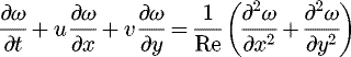 (1)
(1)
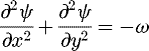 (2)where ψ is the stream function, ω is the vorticity function, u = ∂ ψ/∂ y and v = − ∂ ψ/∂ x are the velocity components, x and y are the Cartesian coordinates, t is the time, and Re is the Reynolds number. In steady cases, the first term of equation (1) will disappear and this equation turns into an elliptic equation same as equation (2) which its solution needs an iterative procedure and known boundary conditions.
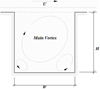 |
Fig. 1 Lid-driven cavity flow geometry. |
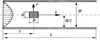 |
Fig. 2 Flow over a square cylinder inside a channel. |
3 Parallel processing on GPUs
In 2006, because of Graphics card's inherent parallel architecture, producers of Graphics cards proposed an idea which, if graphic processors can do a lot of calculation in a moment for image rendering then there is not any problem to process floating point calculations for scientific computing. This idea led to a new parallel processing era and consequently General Purpose GPU (GPGPU) was born during the invention of CUDA by NVIDIA Company. Indeed, CUDA is a parallel computing platform and application programming interface (API) model created by NVIDIA. The CUDA platform is designed to work with programming languages such as C, C++ and Fortran [15]. It should be noted that, in parallel processing literature, GPU and CPU are called device and host, respectively.
In architecture point of view, GPUs have more transistors compared to CPUs. GPUs actually are parallel processors which benefit from huge multithreaded systems. In computer science, a thread is the smallest sequence of programmed instructions that can be managed independently by a scheduler, which is typically a part of the operating system [16]. In a computer CUDA program, a set of commands is named Kernel which looks like a function in other programming languages. When a kernel is called, the instruction of each thread is executed independently. Number of threads which are ready to execute, is set by the programmer in a CUDA code. In parallel processing with GPUs, specified numbers of threads form a larger unit which is called a block. Blocks can be defined in two or more dimensions by the programmer in a CUDA programing code. At last, some blocks make the largest unit of parallel processing structure which is known as grids (see Fig. 3). GPUs and CPUs have two distinct memory spaces which they can not access directly to each other. Every block has a private shared memory which can be accessed only by the threads in that block [17] (see Fig. 4).
In programming on GPUs, instructions are firstly executed by CPU until a kernel is called and at this moment threads begin to execute own instructions. When threads finish their job, again the CPU continues and this procedure is repeated till end of the code (see Fig. 3).
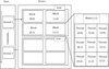 |
Fig. 3 Programming procedure in CUDA. |
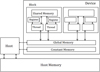 |
Fig. 4 Memory hierarchy in CUDA architecture. |
4 Tridiagonal matrix solvers
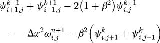
Consider the set of governing equations given by equations (1) and (2). Applying the central difference method on them for the case of steady-state and rearranging the discretized relations, the following formulas in tridiagonal format are obtained: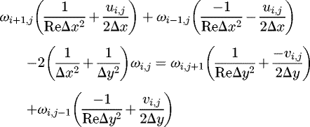 (3)
(3)
 (4)where Δx and Δy are the grid sizes, β = Δx/Δy and i, j are the index of the grid points in the computational grid. For solving the unsteady problem (flow over a square cylinder) the ADI approach is used. In the ADI method each time step splits into two sub-steps i.e. t + Δt/2 and t + Δt. The final discretized equations are given as:
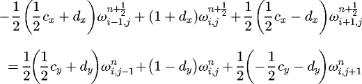 (5)
(5)
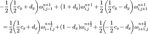 (6)
(6)
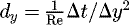
 (7)where c
x
= uΔt/Δx, c
y
= vΔt/Δy,
(7)where c
x
= uΔt/Δx, c
y
= vΔt/Δy, 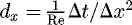 ,
,  , n is the index for time step, and k is the index for iteration. It is well known that the above mentioned equations can be also easily solved by a tridiagonal solver. A tridiagonal matrix solver is an algorithm which calculates unknown vector
  of length n in the system of n equations
  . Here, A is the coefficient matrix of the system of equations (with size of n × n with three non-zero diagonals and
  is a vector of known values. The elements of the main, upper and lower diagonals of matrix A are b
i
,c
i
and a
i
respectively (i = 1, 2, … , n). A variety of ways exist to solve this system of equations where among them the Thomas algorithm is one of the most famous and efficient methods. A brief review of this algorithm and also the CR and PCR algorithms is presented here. Also, the complexity of the algorithms is given in Table 1 [8].
is a vector of known values. The elements of the main, upper and lower diagonals of matrix A are b
i
,c
i
and a
i
respectively (i = 1, 2, … , n). A variety of ways exist to solve this system of equations where among them the Thomas algorithm is one of the most famous and efficient methods. A brief review of this algorithm and also the CR and PCR algorithms is presented here. Also, the complexity of the algorithms is given in Table 1 [8].
4.1 Thomas algorithm
The Thomas algorithm has two stages: (1) forward reduction; (2) backward substitution. In the forward reduction step, the lower diagonal is eliminated sequentially. In this stage equations (8) and (9) are implemented. In stage 2, according to equation (10), all the unknown parameters are evaluated successively.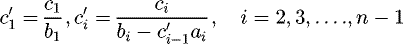 (8)
(8)
 (9)
(9)
 (10)
(10)
As mentioned before, the Thomas algorithm is a sequential algorithm and is not appropriate for parallel computing. To overcome this difficulty, alternative algorithms have been suggested such as cyclic reduction (CR) and parallel cyclic reduction (PCR) for parallel processing applications [4].
4.2 Cyclic reduction algorithm
Like the Thomas algorithm, the CR algorithm has two steps including forward reduction and backward substitution. An overview of the communication pattern for CR algorithm in a 8 × 8 system is illustrated in Figure 5. In the forward reduction phase, CR splits the system of equations into two independent parts with half the number of unknowns, until a system of two unknowns obtains. In each step of forward reduction phase, all even-indexed equations are updated in parallel with equation i, i + 1 and i − 1. Consider that equation i has the form a
i
x
i−1 + b
i
x
i
+c
i
x
i+1 = d
i
, therefore the updated values of coefficients in the forward reduction phase are as follows: (11)
(11)
 (12)where k
1 = a
i
/b
i−1 and k
2 = c
i
/b
i+1. The backward substitution phase calculates the other half of the unknowns using the previously solved values. In each step of the backward substitution phase, all the odd-indexed unknown variables x
i
in parallel by substituting the already solved x
i−1 and x
i+1 values to equation i are solved with respect to equation (13):
(12)where k
1 = a
i
/b
i−1 and k
2 = c
i
/b
i+1. The backward substitution phase calculates the other half of the unknowns using the previously solved values. In each step of the backward substitution phase, all the odd-indexed unknown variables x
i
in parallel by substituting the already solved x
i−1 and x
i+1 values to equation i are solved with respect to equation (13):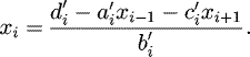 (13)
(13)
An important point is that, CR is applicable only for the system of equations with the size of 2 n which may be the main weakness of this algorithm.
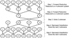 |
Fig. 5 Overview of the communication pattern for CR algorithm in a 8 × 8 system. Superscripts (′) and (″) stand for updated equation. |
4.3 Parallel cyclic reduction algorithm
The PCR algorithm is a modified version of CR algorithm. On the contrary of the CR algorithm, PCR has only one stage, i.e. forward reduction. Another difference between these two algorithms is that PCR utilizes all threads in all levels of the procedure. For example, based on Figure 6 which is related to a 8 × 8 system of equations (each circle shows one row of the equations), after implementing the PCR algorithm twice, four independent sets of equations will be obtained. Finally, each set of equations (which are 2 × 2 is easily solved by an inversing method in parallel. In Figure 7 it can be seen that how PCR works on the matrix of a 4 × 4 system of equations. It should be noted that, similar the CR algorithm, the PCR algorithm is only applicable for a system of equations with the size of 2 n which may be a main weakness.
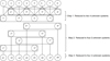 |
Fig. 6 Overview of communication pattern for PCR algorithm in a 8 × 8 system. Superscripts (′) and (″) stand for updated equation. |
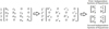 |
Fig. 7 Reduction of a 4 × 4 system of equations into two independent 2 × 2 equations using PCR algorithm. |
5 Implementing Parallel Thomas Approach (PTA) on GPU
Because of the mentioned existing weakness in the CR and PCR algorithms and the sequential Thomas algorithm, in this study another approach for solving tridiagonal system of equations on GPUs is introduced. This is called Parallel Thomas Algorithm (PTA). PTA is the parallel solution of independent tridiagonal systems using the Thomas algorithm. The main idea of this approach is that in a 2D or 3D problem, for an implicit scheme, each computational row of a grid can form an independent tridiagonal system where each of them can be solved by a thread. In other words, each thread solves a tridiagonal matrix independent of the other threads (see Fig. 8 for the thread arrangement). Two main advantages of this approach are that (1) there is no limitation on the size of the system of equations and (2) the implementation and programming is easier than CR or PCR. Note that in many CFD problems, it is hard to fix the size of the computational domain to 2 n and this obstacle could prevent the use of some solving methods such as implicit ones. It is well-known that the Thomas algorithm is a fast and stable algorithm and therefore using many of them simultaneously and in parallel could create a fast method to solve problems.
The used Graphic card in this research is GeForce GTX 580 and the central processor is Intel Corei7 990x Gulf Town. Both graphic and central processors are in the same generation which is an important point that should be considered. The CUDA version is 4.0. In this CUDA version and this hardware with compute capability 2.0 in each direction, blocks cannot exceed from 65535 units. Also in each block the number of threads per blocks has a maximum number of 1024. In the lid-driven cavity problem, the grid dimensions vary from 64 × 64 to 1024 × 1024 and thread per blocks varies from 32 to 256. It is better to set the number of threads per block being a multiple of 32 to manipulate warp capabilities and use the maximum occupancy of threads. All the variables in this research are restored in global memory. According to reference [4] if in the processing of a series of data, all the steps are performed on the GPU, it is not necessary to calculate the first or final data transfer time, but if the GPU is used to boost, only some parts of the process, data transfer time should be considered.
Another aspect in parallel programming using GPUs which is studied here is the “coalesced memory” access. All types of data are stored in memory linearly. For example, the elements of a matrix (v) are stored on global memory as Figure 9. In this figure, the subscripts (n) indicate the row number and superscripts (m) indicate the column number of the matrix. In serial processing, because a processor needs a specific value and reads from a specific location on memory, it is not important how data is stored. But in contrary, in parallel processing, the pattern of thread access to memory is a critical issue. If data access to global memory has a pattern like Figure 9a, it is called “coalesced memory access” and if the memory access has a pattern like Figure 9b, this is called uncoalesced memory access. Figure 9c and d shows two different methods for storing the elements of the tridiagonal matrices (vectors a, b and c) in memory. Here, m is the number of systems and n is dimension of each matrix. The i-th thread is responsible for solving the i-th tridiagonal system. Figure 9c shows the simple storing of the vectors results in a distances of n variables between the corresponding elements in ith and (i + 1)th systems which results in uncoalesced memory access. However, storing the vectors as shown in Figure 9d causes the consecutive threads to access to consecutive data on memory and therefore results in coalesced memory access. Uncoalesced memory access can hurt performance as will be shown for the lid-driven cavity problem in the results section. Due to this, for the second problem (flow over square cylinder), the coalesced memory access is only considered.
The following pseudo-code shows how equation (4) is solved using the PTA algorithm (the pseudo-code for equation (3) is similar to that of equation (4)):
//	m×m is the numerical grid dimension
//	m-2 tridiagonal systems each of which has m-2 unknowns

j = thread number		//	threadIdx.x + blockIdx.x * blockDim.x

0 <= j < m - 2 :

	// lower diagonal
	a[0 + j * (m-2)] = 0
	i : 1 → m - 3
		a[j + i * (m-2)] = -1

	// main diagonal and right-hand side

	i : 0 → m - 3
		q = (i+1)+(j+1)*m
		b[j + i * (m-2)] = 4
		r[j + i * (m-2)] = omega[q]*h^2+psi[q + m]+psi[q - m];

	// upper diagonal
	c[m-3 + j * (m-2)]=0
	i : 0 → m - 4
		c[j + i * (m-2)] = -1

	// forward elimination
	k = j
	cp[k] = c[k] / b[k]
	i : 1 → m - 4
		k = j + i * (m-2);
		cp[k] = c[k] / (b[k]-cp[k - (m-2)]*a[k])

	// backward substitution
	k = j
	dp[k] = r[k] / b[k]
	i : 1 → m - 3
		k = j + i * (m-2)
		dp[k]=(r[k] - dp[k - (m-2)]*a[k]) / (b[k] - cp[k-(m-2)]*a[k])

	// update psi
	i = m - 3
	psi_new[(i+1)+(j+1)*m] = dp[j + i * (m-2)]
	i = m - 4 → 0
		q = (i+1)+(j+1)*m
		k = j + i * (m-2)
		psi_new[q] = dp[k] - cp[k]*psi_new[q+1]
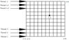 |
Fig. 8 Thread arrangement in parallel Thomas algorithm. |
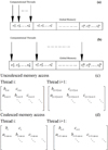 |
Fig. 9 Memory access to global memory (a) Coalesced access (b) Uncoalesced access; Storing traditional matrices for (c) uncoalesced access (d) coalesced access. |
6 Results and discussions
In this study, to assess the PCR, CR, PTA (on GPU), and classic Thomas algorithms (on CPU) and compare their run-times, the steady lid-driven cavity flow and the steady/unsteady flow over a square cylinder inside a channel at various Reynolds numbers are considered. The details of the geometries and governing equations were given in Section 2. The results for the problem of lid-driven cavity flow and for the problem of flow over a square cylinder are presented in Sections 6.1 and 6.2, respectively. In each sub-section, the results obtained using the developed GPU code are verified by the others' well-known References.
6.1 Steady lid-driven cavity flow
Here, the numerical simulation of the steady lid-driven cavity flow at three different Reynolds numbers, i.e., 100, 400 and 1000 is presented. In order to verify the present GPU code, the horizontal velocity component of the flow u(n) the mid-section of the cavity x = 0.5(s) compared to those obtained by Ghia et al. [18] is seen in Figure 10. It can be seen from the figure that the results of the present GPU code are in agreement with the study of Ghia et al. [18]. Therefore, analyzing on the run-time and speed-up is possible.
In order to analyze the runtimes and the performance of PCR, CR, PTA (on GPU), and classic Thomas algorithms (on CPU), the steady lid-driven cavity flow at Re = 1000 s examined for one thousand iterations and different grid sizes from 64 × 64 to 1024 × 1024. The runtimes and speedups of these algorithms are illustrated in Figures 11 and 12, respectively. Here, the speedup of an algorithm is defined as the ratio of its execution time to the runtime of the classic Thomas algorithm. It is evident from Figure 11 that, using PTA (with coalesced memory access) for solving the lid-driven cavity flow in the computational domain of 1024 × 1024 grid size, takes 8.6 seconds (the lowest runtime) and using classic Thomas algorithm takes 331.73 seconds (the highest runtime). In addition, Figure 12 shows that for the CR algorithm, speedup varies between 0.4x and 4.4x for the PCR algorithm, speedup changes from 0.47x to 5.2x and finally for the PTA algorithm (with coalesced memory access), speedup is between 1.7x and 38.45x. These information depict that PTA has the best performance among the other examined methods. The effect of memory access on the run time of the PTA algorithm is also studied for two types of the access pattern, i.e. coalesced and uncoalesced memory accesses. The runtimes and speedups for various grid sizes are shown in Figures 11 and 12. The charts in these figures explain that using the coalesced memory access results about 2x speedup in comparison to the uncoalesced memory access.
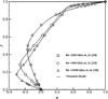 |
Fig. 10 Steady lead-driven cavity flow: horizontal velocity component of the flow (u) the mid-section of the cavity (x = 0.5) for three different Reynolds numbers. |
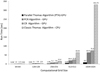 |
Fig. 11 Runtimes of CR, PCR, PTA, and classic Thomas algorithms for the steady lid-driven cavity flow at Re = 1000. |
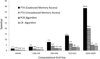 |
Fig. 12 Speedups of CR, PCR, and PTA algorithms for the steady lid-driven cavity flow at Re = 1000. |
6.2 Flow past a square cylinder inside a channel
In this sub-section, the flow over a square cylinder inside a channel, at both steady and unsteady regimes are considered. The relative recirculation length behind square (L c /D) on the steady state regime are compared to the results of Yoon et al. [19] is shown in Figure 13 for Re = 10 ∼ 40. Here, L c is defined as the distance between the square center and the near-wake saddle as indicated by Perry et al. [20]. In unsteady conditions (for example here, Re = 100 the profiles of velocity components (u and v) are plotted along the centerline (i.e. y = 0 and they are compared to those obtained by Breuer et al. [21] is illustrated in Figure 14. In addition, for this test case (i.e. Re = 100 the profiles of u and v at three different axial positions, i.e. x = 0 (center of the cylinder), x = 4 (near-wake), and x = 8 (far-wake) are shown in Figure 15 and are compared to those obtained by Breuer et al. [21]. It can be seen from these examples that the results of the present GPU code are in an excellent agreement with the other studies. Therefore, discussing about the run-time and speed-up is feasible.
The example of lid-driven cavity flow (in the previous sub-section) shows that, PTA (with coalesced memory access) has the best performance among all studied algorithm. Therefore, in this sub-section for analyzing run-time and speed-up, only PTA with coalesced memory access is highlighted. It is worthwhile to present streamlines and vorticity magnitude contours of the flow obtained by the preset GPU code. Figure 16 shows the streamlines of the laminar steady flow for Re = 1, 15a and 30 in which the recirculation lengths are presented in Figure 13 via the solid line. As predicted, for Re < 40 only symmetric recirculation eddies are formed immediately downstream of the cylinder. When Re is increased beyond 40, the wake behind the cylinder becomes unstable. The wake develops a slow oscillation in which the velocity becomes periodic in time and downstream distance, with increasing the amplitude of the oscillation downstream. Figure 17 demonstrates the time-dependent streamlines for Re = 100 at various times, specifically at t =100,102, 104, 106, 108 and 110 seconds. Also in Figure 18 the patterns of vorticity behind the cylinder for four different Reynolds numbers i.e. Re = 75, 100, 150 and 200 at t = 100 s are presented. The figure shows that the oscillating wake rolls up into two staggered rows of vortices with opposite sense of rotation. Because of the similarity of the wake with the footprints in a street, staggered rows of vortices behind the square cylinder is called as Von-Karman vortex Street. Eddies periodically break off alternately from two sides of the cylinder as seen in Figure 18. In addition, the variation of Strouhal number (St = fD/U max ) computed by the cylinder diameter D the measured frequency of the vortex shedding f and the maximum velocity U max at the channel inflow plane, versus Reynolds number (Re) is shown in the lower part of Figure 18. The results are also compared to those obtained by Breuer et al. [21] via a finite volume method.
The final result presents the effect of using PTA with coalesced memory access on execution times of the unsteady flow simulation. For this purpose, the runtimes and speedups of PTA for the unsteady flow across a square cylinder at Re = 100 and Re = 200 on three different grid sizes (i.e. 160 × 800, 200 × 1000, and 400 × 2000 are obtained and illustrated in Figure 19. The figure shows that PTA can decrease the time of simulation even for an unsteady flow and this time reduction would be more considerable when the computational grid points increase (as the increase of computational grid points is necessary to make results more precise).
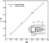 |
Fig. 13 Recirculation length behind the square in steady state regime. |
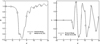 |
Fig. 14 Comparison of the velocity profile along the centerline (i.e. y = 0) at Re = 100: (a) streamwise velocity, u. (b) Cross-stream velocity, v. |
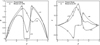 |
Fig. 15 Comparison of the velocity profile at three different positions in the flow field, center of cylinder (x = 0) near wake (x = 4) and far-wake (x = 8) at Re = 100 (a) streamwise velocity, u. (b) Cross-stream velocity, v. |
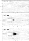 |
Fig. 16 Streamlines of the laminar steady flow over the square cylinder for Re=1, 15 and 30. |
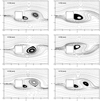 |
Fig. 17 Streamlines of the laminar unsteady flow over the square cylinder for Re = 100 at =100, 104, 106, 108 and 110 seconds. |
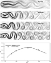 |
Fig. 18 Vorticity magnitude contours of the laminar unsteady flow over the square cylinder for Re = 75, 100, 150 and 200 at t = 100s. The variation of Strouhal number (St) versus Reynolds number (Re). |
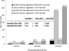 |
Fig. 19 Runtimes and speedups of PTA for the unsteady flow over a square cylinder at Re = 100 and Re = 200 on different grid sizes. |
7 Conclusion
In this research a modified approach for solving tridiagonal system of equations on GPUs is introduced which is called Parallel Thomas Algorithm (PTA). Firstly, a comparison between PTA and two conventional parallel algorithms i.e. CR and PCR (both on GPU) as well as the serial processing solver (i.e. classic Thomas algorithm on CPU) is performed by simulating the lid-driven cavity flow. In addition, the issue of coalesced and uncoalesced memory access and its effect on the speedups are studied. The results show that the speedup of CR, PCR and PTA against CPU runtime (classic Thomas algorithm) is around 4.4x, 5.2x and 38.5x, respectively. Also, the effect of coalesced memory access and uncoalesced memory access to global memory is also examined, and a 2x speedup is achieved in coalesced memory access on GPU. In addition, to assess PTA performance in time dependent problems, the unsteady flow over a square cylinder is solved and a speedup around 9x is obtained against CPU-runtime.
Nomenclature
D : Length and width of the square [m]
f : Frequency of the vortex shedding [Hz]
H : Height of the cavity or channel [m]
i, j : Index of the grid points [–]
L : Length of the computational domain [m]
u : Horizontal velocity component [m s−1]
v : Vertical velocity component [m s−1]
References
- B. Tutkun, F.O. Edis, A GPU application for high-order compact finite difference scheme, Comput. Fluids 55, 29–35 (2012) [Google Scholar]
- V. Esfahanian, H. Mahmoodi Darian, S.M.I. Gohari, Assessment of WENO schemes for numerical simulation of some hyperbolic equations using GPU, Comput. Fluids 80, 260–268 (2013) [Google Scholar]
- H. Mahmoodi Darian, V. Esfahanian, Assessment of WENO schemes for multi-dimensional Euler equations using GPU, Int. J. Numer. Meth. Fl. 76, 961–981 (2014) [CrossRef] [Google Scholar]
- Y. Zhang, J. Cohen, J.D. Owens, Fast tridiagonal solvers on the GPU, in Proceedings of the 15th ACM SIGPLAN Symposium on Principles and Practice of Parallel Programming, Bangalore , January 9–14 (2010) 127–136 [Google Scholar]
- D. Egloff, High performance finite difference PDE solvers on GPUs, Technical report, QuantAlea GmbH, February, 2010 [Google Scholar]
- D. Göddeke, R. Strzodka, Cyclic reduction tridiagonal solvers on GPUs applied to mixed-precision multigrid, IEEE Trans. Parallel Distrib. Syst. 22, 22–32 (2011) [Google Scholar]
- A. Davidson, Y. Zhang, J.D. Owens, An auto-tuned method for solving large tridiagonal systems on the GPU, Proceedings of the 25th IEEE Intern. Parallel and Distributed Processing Symposium, Anchorage, Alaska, 16–20 May (2011) 956–965 [Google Scholar]
- H.S. Kim, S. Wu, W.L. Chang, W.M.W. Hwu, A scalable tridiagonal solver for GPUs, in Inter. Conf. on Parallel Processing, Taipei City (September 2011) 444–453 [Google Scholar]
- P. Quesada-Barriuso, J. Lamas-Rodríguez, D.B. Heras, M. Bóo, F. Argüello, Selecting the best tridiagonal system solver projected on Multi-Core CPU and GPU platforms, in 17th International Conference on Parallel and Distributed Processing Techniques and Applications, Las Vegas, Nevada, USA, 18–19 July, 2011 [Google Scholar]
- V. Esfahanian, B. Baghapour, M. Torabzadeh, H. Chizari, An efficient GPU implementation of cyclic reduction solver for high-order compressible viscous flow simulations, Comput. Fluids 92, 160–171 (2014) [Google Scholar]
- M. Giles, E. Laszlo, I. Reguly, J. Appleyard, J. Demouth, GPU implementation of finite difference solvers, in Seventh Workshop on High Performance Computational Finance, New Orleans, LA, USA , 16–17 November, 2014 [Google Scholar]
- H.J. Macintosh, D.J. Warne, N.A. Kelson, J.E. Banks, T.W. Farrell, Implementation of parallel tridiagonal solvers for a heterogeneous computing environment, ANZIAM J. 56, 446–462 (2016) [CrossRef] [Google Scholar]
- K. Karimi, N.G. Dickson, F. Hamze, A performance comparison of CUDA and OpenCL, The Computing Research Repository, https://arxiv.org/abs/1005.2581 [Google Scholar]
- J. Fang, A.L. Varbanescu, H. Sips, A comprehensive performance comparison of CUDA and OpenCL, International Conference on Parallel Processing (ICPP), Taipei, Taiwan, 13–16 September, 2011 [Google Scholar]
- NVIDIA CUDA Home Page: https://developer.nvidia.com/cuda-zone [Google Scholar]
- L. Lamport, How to make a multiprocessor computer that correctly executes multiprocess programs, IEEE Trans. Comput. C28, 690–691 (1979) [Google Scholar]
- G. Vasiliadis, S. Antonatos, M. Polychronakis, E.P. Markatos, S. Ioannidis, Gnort: high performance network intrusion detection using graphics processors, in Proceedings of the 11th International Symposium on Recent Advances in Intrusion Detection (RAID), Cambridge, MA, USA , September 15–17, 2008 [Google Scholar]
- U. Ghia, K.N. Ghia, C.T. Shin, High-Re solutions for incompressible flow using the Navier-Stokes equations and a multigrid method, J. Comput. Phys. 48, 387–411 (1982) [Google Scholar]
- D.H. Yoon, K.S. Yang, C.B. Choi, Flow past a square cylinder with an angle of incidence, Phys. Fluids 22, 043603 (2010) [CrossRef] [Google Scholar]
- A.E. Perry, M.S. Chong, T.T. Lim, The vortex-shedding process behind two-dimensional bluff bodies, J. Fluid Mech. 116, 77–90 (1982) [Google Scholar]
- M. Breuer, J. Bernsdorf, T. Zeiser, F. Durst, Accurate computations of the laminar flow past a square cylinder based on two different methods: Lattice-Boltzmann and finite-volume, Int. J. Heat Fluid Fl. 21, 186–196 (2000) [CrossRef] [Google Scholar]
Cite this article as: M. Souri, P. Akbarzadeh, H.M. Darian, Parallel Thomas approach development for solving tridiagonal systems in GPU programming − steady and unsteady flow simulation, Mechanics & Industry 21, 303 (2020)
All Tables
All Figures
|
Fig. 1 Lid-driven cavity flow geometry. |
| In the text | |
|
Fig. 2 Flow over a square cylinder inside a channel. |
| In the text | |
|
Fig. 3 Programming procedure in CUDA. |
| In the text | |
|
Fig. 4 Memory hierarchy in CUDA architecture. |
| In the text | |
|
Fig. 5 Overview of the communication pattern for CR algorithm in a 8 × 8 system. Superscripts (′) and (″) stand for updated equation. |
| In the text | |
|
Fig. 6 Overview of communication pattern for PCR algorithm in a 8 × 8 system. Superscripts (′) and (″) stand for updated equation. |
| In the text | |
|
Fig. 7 Reduction of a 4 × 4 system of equations into two independent 2 × 2 equations using PCR algorithm. |
| In the text | |
|
Fig. 8 Thread arrangement in parallel Thomas algorithm. |
| In the text | |
|
Fig. 9 Memory access to global memory (a) Coalesced access (b) Uncoalesced access; Storing traditional matrices for (c) uncoalesced access (d) coalesced access. |
| In the text | |
|
Fig. 10 Steady lead-driven cavity flow: horizontal velocity component of the flow (u) the mid-section of the cavity (x = 0.5) for three different Reynolds numbers. |
| In the text | |
|
Fig. 11 Runtimes of CR, PCR, PTA, and classic Thomas algorithms for the steady lid-driven cavity flow at Re = 1000. |
| In the text | |
|
Fig. 12 Speedups of CR, PCR, and PTA algorithms for the steady lid-driven cavity flow at Re = 1000. |
| In the text | |
|
Fig. 13 Recirculation length behind the square in steady state regime. |
| In the text | |
|
Fig. 14 Comparison of the velocity profile along the centerline (i.e. y = 0) at Re = 100: (a) streamwise velocity, u. (b) Cross-stream velocity, v. |
| In the text | |
|
Fig. 15 Comparison of the velocity profile at three different positions in the flow field, center of cylinder (x = 0) near wake (x = 4) and far-wake (x = 8) at Re = 100 (a) streamwise velocity, u. (b) Cross-stream velocity, v. |
| In the text | |
|
Fig. 16 Streamlines of the laminar steady flow over the square cylinder for Re=1, 15 and 30. |
| In the text | |
|
Fig. 17 Streamlines of the laminar unsteady flow over the square cylinder for Re = 100 at =100, 104, 106, 108 and 110 seconds. |
| In the text | |
|
Fig. 18 Vorticity magnitude contours of the laminar unsteady flow over the square cylinder for Re = 75, 100, 150 and 200 at t = 100s. The variation of Strouhal number (St) versus Reynolds number (Re). |
| In the text | |
|
Fig. 19 Runtimes and speedups of PTA for the unsteady flow over a square cylinder at Re = 100 and Re = 200 on different grid sizes. |
| In the text | |
Current usage metrics show cumulative count of Article Views (full-text article views including HTML views, PDF and ePub downloads, according to the available data) and Abstracts Views on Vision4Press platform.
Data correspond to usage on the plateform after 2015. The current usage metrics is available 48-96 hours after online publication and is updated daily on week days.
Initial download of the metrics may take a while.