| Issue |
Mechanics & Industry
Volume 21, Number 3, 2020
|
|
|---|---|---|
| Article Number | 302 | |
| Number of page(s) | 14 | |
| DOI | https://doi.org/10.1051/meca/2020019 | |
| Published online | 03 April 2020 | |
Regular Article
Effect of hardening law and process parameters on finite element simulation of single point incremental forming (SPIF) of 7075 aluminum alloy sheet
1
Department of Integrated Systems Engineering, The Ohio State University, 210 Baker Systems, 1971 Neil Avenue, Columbus, OH 43210, USA
2
Department of Mechanical and Aerospace Engineering, The Ohio State University, 201 W 19th Ave, Columbus, OH 43210, USA
3
Department of Automotive Engineering, Clemson University, Greenville, SC 29607, USA
* e-mail: This email address is being protected from spambots. You need JavaScript enabled to view it.
Received:
15
May
2019
Accepted:
27
February
2020
Abstract
In the last two decades, the advances of using computers in sheet metal forming processes have introduced a novel adjustable process known as incremental sheet forming (ISF) as an optimal method for fast prototyping and low numbers of production. Formability and deformation behavior of ISF process are highly affected by the selected process parameters, such as the toolpath, step size, tool diameter, feed rate, and lubrication. The purpose of this work was to study the effect of these process parameters as well as hardening law on single point incremental forming (SPIF) process. For this work, a truncated-cone geometry was considered as a target shape with 7075-O aluminum alloy sheets. The simulations were conducted with different process parameters, i.e., toolpath type, step size, tool size, feed rate, friction coefficient, and wall angle with respect to the tool force and moment, effective plastic strain distribution and thickness of the part. In addition, three types of hardening laws i.e., isotropic extended Voce type hardening law, combined isotropic-kinematic Chaboche type hardening laws with single and double back-stress terms were applied in the finite element simulation of SPIF process. A detailed comparison of these hardening laws' predictions was made with respect to the tool force and moment, effective plastic strain distribution and thickness of the part.
Key words: Combined isotropic-kinematic hardening law / Chaboche / ISF process parameters / incremental sheet forming / SPIF / toolpath
© AFM, EDP Sciences 2020
1 Introduction
Recent advances of using computers in sheet metal forming processes have led to novel adjustable forming techniques evolved from conventional processes like stamping. One of these upcoming techniques is incremental sheet forming (ISF) process. In ISF process, the sheet metal is gradually being formed by at least one CNC operated forming tool with many additive local deformations [1–3]. This technique does not need any dedicated punches or dies [1,4], and conveys the appropriate amount of plastic deformations to the sheet which produces the final form of the part. Due to the ISF method adjustability, forming extensive 3D contours is possible [5,6]. In this process, at least a cylindrical tool with hemispherical head contacts the sheet metal, and plastically deforms it at the contact point. Then, by moving the tool following a predetermined path, part is gradually formed [7,8].
Common configurations of ISF are:
-
Single point incremental forming (SPIF), in which the sheet is formed using a single indenter [9].
-
Double sided incremental forming (DSIF), in which the sheet is formed using two indenters on both sides of the sheet [10].
-
Two point incremental forming (TPIF), in which the sheet is formed against a male or a female partial or full die [11].
In a review by Esmaeilpour et al. on ISF process, fundamental deformation mechanism, formability, and important topics were discussed in detail. It was mentioned that a combination of deformation modes i.e., bending, stretching and shear are involved in the ISF process. Each deformation mode contribution is highly affected by the selected process parameters [1]. Using many experiments, Ham and Jeswiet checked the impact of feed rate, spindle rotation speed, step size and wall angle on forming a part [12]. Based on a study by Bhattacharya et al., formability decreases by using larger tool diameter and step size, and decreasing the sheet thickness. They also reported that feed rate does not have a significant impact on the formability. [13]. In a study by Petek et al., larger deformations and forces were reported by increasing the wall angles, step sizes and tool sizes. However, lubrication and tool rotation do not have meaningful effect on forces and maximum strains [14]. According to several studies, the formability improves by having a larger value of the step size in small range of step sizes, and it reduces for higher range of the step sizes. However, more studies are still required to investigate the impact of step size on formability as some other researchers mentioned that the formability is not affected by step size. It was also mentioned that increasing the tool rotation and decreasing the tool feed rate will provide a better formability. However, these effects should also be studied in more detail [1].
Beside the experimental studies on ISF process, modeling of this method is also essential to provide a better view of the deformation behavior. As the contact condition is changing fast in ISF process, it is computationally time-consuming to be modeled with implicit or explicit finite element codes [15,16]. In a study by Yamashita et al. on the dynamic explicit FE modeling of the ISF method, it was concluded that numerical simulation could be applied for the optimization of this process [17]. The use of a material model for the ISF process has also been investigated by several researchers. Yield functions, such as von Mises and Hill's 1948 were widely used by researchers [18,19]. However, predicted shapes using these two yield functions are almost identical as mentioned in a study by Bambach and Hirt [20]. With respect to the choice of material model in the ISF process, comparison of three different yield functions namely; Yld2004-18p, Hill's 1948, and von Mises were made in previous studies by the authors. It was concluded that due to through-the-thickness shears, applying a 3D yield function, such as Yld2004-18p is imperative to account for shear and normal stress components. However, for the SPIF process, since predicted strain histories were very similar for different yield functions, the von Mises yield criterion was recommended due to its simplicity and a lower computational time [21–23]. The choice of hardening laws, such as isotropic, kinematic or mixed models, has an important effect on the force prediction in ISF processes. However, the effect of using different types of kinematic and mixed models should be studied in more details as mentioned in a review paper on incremental forming process [1].
A better view of the deformation mechanics in ISF processes is achievable by investigating the forming forces. In a study by Cerro et al., it was reported that by increasing the step size, tool size, wall angle or sheet thickness, the forming forces increase. However, step size has the least impact which can be increased without a great penalty to decrease the production time [24]. Saidi et al. studied the influence of several parameters on the evolution of the axial forming force during the incremental forming of a truncated cone. They were able to optimize the process with respect to the most influent parameters [25]. In previous studies by the authors, it was shown that predicted forces are affected by the choice of yield functions [22,23]. In a study by Doflou et al. on SPIF process, it was reported that a linear fit provides accurate approximations for the forces in different step sizes and tool sizes. In addition, they provided quadratic fits of the force trends for different sheet thicknesses and wall angles [26]. In another study, it was noticed that the tangential force increases by having a larger sheet thickness, step size and wall angle [27].
The purpose of this study was to investigate the effect of process parameters and different types of hardening models on SPIF process. For this reason, in the SPIF simulation of 7075-O aluminum alloy sheet, the impact of toolpath type, tool size, step size, feed rate, friction coefficient, and wall angle were studied with respect to the tool force and moment, effective plastic strain distribution and thickness of the part. In addition, three types of hardening models i.e., isotropic extended Voce, combined isotropic-kinematic Chaboche with one back-stress term, and combined isotropic-kinematic Chaboche with two back-stress terms were applied in the finite element simulation of SPIF process. A comparison of the three hardening laws' predictions was performed regarding the tool force and moment, effective plastic strain distribution and thickness of the part.
In the next section, description of tensile and TCT tests will be presented. In Section 3, the FE modeling of SPIF will be investigated as a function of process parameters and different hardening models. At the end, in Section 4, conclusions will be discussed.
2 Uniaxial tensile and TCT tests
In a previous study by the authors, uniaxial tensile tests of 30 mm gauge length dog-bone specimens were performed to obtain the macroscopic flow stress behavior of AA7075-O [23]. The specimens were cut and prepared using water-jet based on ASTM E8 [28]. Tensile tests were conducted using an electro-mechanical universal load frame INSTRON 5985. ARAMIS 5M, a 3D digital image correlation (DIC) system, was utilized to monitor the deformation of the specimens at a constant rate of 10 fps. 10 mm/min crosshead speed was set for all the tests. For anisotropy, the tensile tests were conducted in the rolling, diagonal and transverse directions at room temperature. The engineering stress–strain curves are presented in Figure 1.
In addition, the in-plane cyclic loading experimental device was used to measure hardening curves in tension-compression-tension (TCT) tests, as shown in Figure 2. The system was mounted on an electro-mechanical INSTRON load frame, fitted with 100kN load cell. The specimen was bolted on the grips, attached to the load frame. The thickness direction of the specimen gauge area was painted with black and white speckle pattern to be tracked by the DIC system. The DIC system not only records the strain on a pre-defined virtual extensometer in real-time, but also provides feedback to the load frame to control the change in the loading directions according to the pre-defined cyclic loading pattern. The main highlight of this setup was the anti-buckling technique during the compression tests. The specimen was held in the thickness direction between two plates using pneumatic force. The side plates were attached to a small 2000 lb load cell to record the magnitude of side forces on the specimen. The whole frame was mounted on guided rails which can be automatically self-centered to accommodate the change in material thickness during the test. To reduce errors caused by friction forces induced by the anti-buckling side plates, two layers of Teflon with a thickness of 0.1 mm were attached on the surface of each anti-buckling block, and a lubricant was sprayed on them before the test. The specimens were machined to a gauge length of 20 mm and a gauge width of 10 mm, which referred to the optimal anti-buckling specimen design suggested by Boger et al. [29]. The measured stress-strain curves for the TCT tests are shown in Figure 28.
 |
Fig. 2 Setup of conducting in-plane cyclic loading experiments. |
3 FE simulation of SPIF process
3.1 FEM base conditions
A truncated-conical geometry with 140 mm base diameter and 55 mm depth was considered for finite element simulation of the SPIF process. The initial sheet blank with 1.6 mm thickness has a circular shape with a 90 mm radius and mechanical properties of 2.81E–9 ton/mm3 density, E = 71.1 GPa and v = 0.33 [30]. To investigate the effect of anisotropic material models on ISF process, a comparison of three various yield functions, Yld2004-18p, Hill's 1948, and von Mises were made in previous studies by the authors. It was concluded that due to through-the-thickness shears, applying a 3D yield function, such as Yld2004-18p is paramount to account for shear and normal stress components. However, for the SPIF process, since predicted strain histories were very similar for different yield functions [22,23], von Mises yield criterion was used instead in this study due to its simplicity and a lower computational time. In the simulation of the SPIF process, using solid elements to account for full 3D stress components are more appropriate than using shell type elements [1,31]. To model the blank sheet, 87,773 reduced integration 8-node brick solid elements (C3D8R) with 0.7 mm × 0.7 mm × 0.5333 mm (through-thickness) dimensions were used in ABAQUS utilizing 24 CPU processors, E5-2630, with 2.3GHz speed. In this study, fixed boundary conditions are preferred over modeling the blank clamping process to save the computational time as mentioned in a study by Kim et al. [32]. The tool with a hemispherical head was assumed as a rigid surface. The surface-to-surface contact was considered for the tool and the sheet. To further reduce the computational time, 107 mass scaling factor was considered for all cases. Due to the quasi-static nature of the process, and based on the ABAQUS manual [33], the ratio of the kinetic energy to internal energy was monitored to ensure that it is less than 10%. For all simulations, the kinetic energy was almost negligible compared to the internal energy which guaranteed that the mass-scaled simulations are still under the quasi-static condition. All the above conditions were then fixed for all simulation cases considered in this study.
The following baseline values were used for geometrical parameters: 67° for the wall angle of the truncated-conical geometry, and 12.7 mm diameter for the hemispherical head of the tool. Using a MATLAB code, a spiral type toolpath was generated to produce the truncated-cone geometry with 50 mm/s feed rate, and 0.927 mm step size. A Coulomb friction coefficient of 0.1 was assumed for the contact of sheet and tool, which is commonly used to represent for the well lubrication of sheet forming processes. In addition, like the previous study by the authors, the Voce type hardening model was applied since it accurately represents the hardening behavior of the aluminum alloy sheet. The coefficients of the Voce type hardening law were calculated previously [23] using the true stress-strain data in RD: (1)where
  is in MPa.
3.2 Effect of different types of toolpath on FE simulation of SPIF process
Toolpath defines movement contours of the tool which affects the contact condition between the sheet and the tool, and consequently affects the distribution of the strain and stress. As a result, geometric accuracy and the formability of the material will be affected which means optimal tool paths are required in ISF processes to provide desirable range of geometric design features and formability in the formed product [34]. One decent choice for ISF application is the z-level (profile) tool path. Any complicated geometry can be produced using this type of tool path. However, this toolpath commonly leaves a scarring on the surface of the formed part. This can be remedied by pushing the scar to the edge of the formed part. Due to the rapid transition between following contours, helical (spiral) tool path completely removes the surface scarring and generates homogeneous thinning which makes it a decent tool path for the ISF process [35,36]. Helical and profile tool paths are presented in Figure 3.
In this part of the study, two types of toolpath were applied in the FE simulation of SPIF method to produce a truncated-conical geometry. For this purpose, a MATLAB code was written to provide these two types of toolpath in Abaqus. Then, SPIF process was applied to produce a truncated-conical geometry as explained in Section 3.1. Figure 4 presents the distributions of effective strain in SPIF simulations for the top element layer of the sheet metal which is in contact with the tool for spiral and Z-level toolpath types. Although these two contours are identical in most of the formed part, the contour for the Z-level toolpath type shows a line of severe localized effective strain distribution which represents the scarring on the surface caused by upward/downward transition between the following contours. Figures 5 and 6 display the tool reaction force and moment for spiral and Z-level toolpath types, respectively. The amount of the tool reaction force and moment is almost identical for different toolpath types. The excessive thinning causing failure in the sheet metal is an important consideration in the ISF process. The thickness was determined as the distance between the inner and outer sheet surface along the normal to the surface in contact with the tool. The calculated thickness of the part based on spiral and Z-level toolpath types are shown in Figure 7. More thinning can be seen in the Z-level toolpath type, which means this type of toolpath has a higher chance of failure. The minimum thickness in the formed part by the Z-level toolpath type is about 0.4 mm while the minimum thickness is about 0.5 mm for the spiral toolpath type. The initial thickness before the deformation for both types of toolpaths was 1.6 mm.
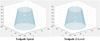 |
Fig. 3 Common ISF tool paths: left) Spiral (Helical) type tool path, right) Z-Level (Profile) type tool path. |
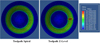 |
Fig. 4 Effective strain distribution of sheet metal using different toolpath types. |
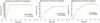 |
Fig. 5 Tool reaction force by different toolpath types. |
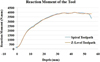 |
Fig. 6 Tool reaction moment by different toolpath types. |
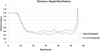 |
Fig. 7 Thickness-depth distribution for different toolpath types. |
3.3 Effect of different step sizes on FE simulation of SPIF process
The step size is the distance between contours in tool axis direction. Generally, decreasing step size can improve the material forming limit as a larger step size will generate a pulling effect due to a large tensile force along the wall which compromise the stabilization effect from the bending in the contact area. In this part, three different step sizes in the FE simulation of SPIF method were applied in producing a truncated-conical geometry as explained in detail in Section 3.1. Figure 8 presents effective strain distributions of the sheet metal for different step sizes. Although these contours are identical in most parts, the contour for the smallest step size shows a higher effective strain distribution in some areas. Figures 9 and 10 display the tool reaction force and moment for different step sizes, respectively. The magnitude of tool reaction force and moment is higher for larger step sizes. The lowest forming forces and the highest effective strain distribution are observed for the smallest step size which means it provides a better formability in comparison to the larger step sizes. These results show good agreement with the work on AA3003 by Ham and Jeswiet [12]. Although a smaller step size provides a better formability, it increases the processing time and consequently the cost of production. The calculated thickness distribution based on different step sizes is shown in Figure 11 which is almost identical for different step sizes. The minimum thickness in some locations in the formed part is about 0.5 mm while the initial thickness was 1.6 mm.
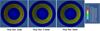 |
Fig. 8 Effective strain distribution of sheet metal using different step sizes. |
 |
Fig. 9 Tool reaction force by different step sizes. |
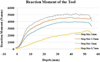 |
Fig. 10 Tool reaction moment by different step sizes. |
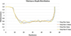 |
Fig. 11 Thickness-depth distribution for different step sizes. |
3.4 Effect of different tool sizes on FE simulation of SPIF process
In this part, three different tool sizes were used in the FE simulation of SPIF method to produce a truncated-conical geometry, as explained in Section 3.1. Figure 12 presents effective strain distributions of the sheet metal for different tool sizes. The contour for the smallest tool size shows a higher effective strain distribution. Figures 13 and 14 show the tool reaction force and moment for different tool sizes, respectively. The amount of tool reaction force and moment is higher for larger tool sizes due to the larger contact area between the sheet and the tool. The lowest forming forces and the highest effective strain distribution can be seen for the smallest tool size which means it provides a better formability in comparison to the larger tool sizes. The calculated thickness distribution based on different tool sizes is shown in Figure 15 which is almost identical for different tool sizes. However, in some parts, more thinning can be seen for larger tool which means it has a higher chance of failure. These results show a good agreement with the work by Gheysarian and Honarpisheh [37].
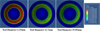 |
Fig. 12 Effective strain distribution of sheet metal using different tool sizes. |
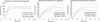 |
Fig. 13 Tool reaction force by different tool sizes. |
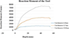 |
Fig. 14 Tool reaction moment by different tool sizes. |
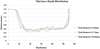 |
Fig. 15 Thickness-depth distribution for different tool sizes. |
3.5 Effect of different feed rates on FE simulation of SPIF process
The feed rate changes the friction condition between the sheet and the tool. It also affects the strain rate of material deformation. In this part, the effect of different feed rates was studied. Figure 16 presents effective strain distributions in the sheet metal for different feed rates. As can be seen, they look very similar. Figures 17 and 18 show the tool reaction force and moment for different feed rates, respectively, which are almost identical. The calculated thickness distribution based on different feed rates is also shown in Figure 19 which is almost similar for different feed rates. In conclusion, the feed rate does not have a significant effect on the SPIF process for the AA7075-O aluminum sheet, which is considered as a strain-rate insensitive material. However, feed rate does have an effect on the total process time and surface quality. The slight differences in the simulation results are mainly caused by the dynamic effect which depends on the tool feed rate.
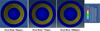 |
Fig. 16 Effective strain distribution of sheet metal using different feed rates. |
 |
Fig. 17 Tool reaction force by different feed rates. |
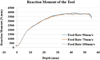 |
Fig. 18 Tool reaction moment by different feed rates. |
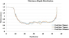 |
Fig. 19 Thickness-depth distribution for different feed rates. |
3.6 Effect of friction coefficients on FE simulation of SPIF process
Friction generates heat which affects the material microstructure as well as surface quality. It also has an impact on the through-thickness-shear which might affect the material formability. For comparison, a baseline friction coefficient of 0.1 was used in the SPIF simulation, since it represents a well lubricated tool-work piece contact surface. Also, three different friction coefficients i.e., 0.05, 0.1 and 0.2 were used in the finite element simulation of SPIF process to represent various lubrication conditions. Figure 20 shows effective strain distributions of the sheet metal for different friction coefficients. These contours look similar for different friction coefficients. Figures 21 and 22 present the tool reaction force and moment for different friction coefficients. The amount of the in-plane reaction force and moment are higher for larger friction coefficient. The thickness distribution is plotted in Figure 23 which is almost identical for different friction coefficients. It can be concluded that although friction coefficient might affect surface quality, it does not have a considerable effect on formability in the SPIF process.
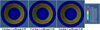 |
Fig. 20 Effective strain distribution for different friction coefficients. |
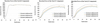 |
Fig. 21 Tool reaction force by different friction coefficients. |
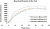 |
Fig. 22 Tool reaction moment by different friction coefficients. |
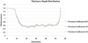 |
Fig. 23 Thickness-depth distribution for different friction coefficients. |
3.7 Effect of wall angles on FE simulation of SPIF process
In this part, three different wall angles were investigated in the FE simulation of SPIF method. Figure 24 presents effective strain distributions of the sheet metal for different wall angles. The contour for the larger wall angle shows a higher effective strain distribution. Figures 25 and 26 show the tool reaction force and moment for different wall angles. The amount of the in-plane reaction forces and the moment of the tool are greater for larger wall angle which is to be expected. The calculated thickness distribution based on various wall angles is presented in Figure 27 which shows thinner thickness for larger wall angle. This can also be explained by the sine law, a simple mathematical expression to estimate the thinning of the sheet metal based on the geometry of tool. The relationship between the original sheet thickness, t
0, and the current thickness, t
1, as a function of a given wall angle, α, is given by [38]: (2)
(2)
Calculated thicknesses from the simulation as well as the sine law are presented in Table 1 for different wall angles. As can be seen, the calculated thickness from the simulation is very close to the reported one by the sine law for all cases. The thickness for the formed sheet with a 75° wall angle is less than 0.4 mm in some areas while the minimum thickness for the formed sheet with a 60° wall angle is more than 0.6 mm. The initial thickness before the deformation for different wall angles was 1.6 mm. Higher thinning for larger wall angles means that increasing the wall angle increases the chance of an earlier failure.
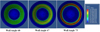 |
Fig. 24 Effective strain distribution of sheet metal using different wall angles. |
 |
Fig. 25 Tool reaction force by different wall angles. |
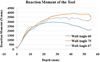 |
Fig. 26 Tool reaction moment by different wall angles. |
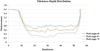 |
Fig. 27 Thickness-depth distribution for different wall angles. |
Thickness for different wall angles.
3.8 Effect of different types of hardening model on FE simulation of SPIF process
In this part, three types of hardening laws were considered in the finite element simulation of SPIF process. The first one is the extended Voce type isotropic hardening model, as following [39]: (3)where
  is an effective (or equivalent) stress in MPa. A, B, p, C and q are the hardening parameters which were determined based on the true stress-strain curve measured in the rolling direction up to the uniform deformation limit. The calculated parameters are listed in Table 2. The second and third hardening models are based on Chaboche type combined isotropic kinematic hardening model with one and two back-stress terms, respectively. Isotropic part was described in equation (3). The following shows the back-stress (α) evolution:
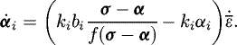 (4)
(4)
The subscript i represents the number of back-stress term. f is the yield function which is von-Mises isotropic yield function in this study. k and b are the parameters controlling the back-stress evolution and were obtained using the stress–strain curves in the tension-compression-tension (TCT) tests. The results are summarized in Table 2. Figure 28 presents the comparison of the three calibrated hardening models with the experimental stress-strain curve in TCT tests, as explained in Section 2. It was found that the extended Voce type isotropic hardening model accurately accounts for the hardening behavior of the sheet metal only in the initial tension part, while most of the TCT test results are well captured by the Chaboche type hardening models. The Chaboche model with two back-stress terms shows the best prediction especially for the transition part between the elastic and plastic part.
Table 2 presents the calibrated parameters for extended Voce, Chaboche with single and double back-stress terms:
Figure 29 presents effective strain distributions of the sheet metal for extended Voce, Chaboche with single and double back-stress terms. The contour plots show more severe effective strain distributions for Chaboche with single and double back-stress terms, which is due to a lot of loading and unloading involved in the SPIF process. Figures 30 and 31 present the tool reaction force and moment for three hardening models. The amount of tool reaction force and moment are greater for extended Voce which is due to the differences between these hardening models in predicting path changes involved in repeated loading and unloading processes. The thickness distributions for the three hardening models are similar as presented in Figure 32.
Material parameters of hardening models used in this study.
 |
Fig. 28 TCT stress–strain curve experiment vs. extended Voce, Chaboche with one back-stress term, and Chaboche with two back-stress terms. |
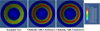 |
Fig. 29 Effective strain distribution of sheet metal using different hardening models. |
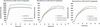 |
Fig. 30 Tool reaction force by different hardening models. |
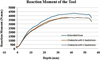 |
Fig. 31 Tool reaction moment by different hardening models. |
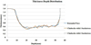 |
Fig. 32 Thickness-depth distribution for different hardening models. |
4 Conclusion
In this paper, FE simulation was utilized to investigate the effect of process parameters and the hardening models on the single point incremental sheet forming (SPIF) of a truncated cone with 7075-O aluminum alloy sheet. Specifically, the effects that toolpath type, feed rate, step size, friction coefficient, tool size, and wall angle have on the tool force and moment, effective plastic strain distribution and thickness of the part were studied.
-
It was concluded that spiral toolpath is the best choice to form simple geometries, such as cones, as effective strain distribution was seen to be more uniform due to the gradual movement of tool in upward/downward transition which provides a better quality of the surface. Furthermore, less thinning was seen for this type of toolpath which postpones the risk of failure in comparison to the Z-level toolpath. However, forces and moments of the tool were not affected by the choice of toolpath.
-
It was shown that smaller tool size and step size provide a better formability. However, to have a decent surface quality, they should be optimized.
-
It was concluded that while friction coefficient and feed rate are important to have a better surface quality, they do not have a considerable effect on formability in the SPIF process.
-
As for anisotropic material properties, the effect of the yield function was reported trivial in previous studies by the authors [22,23]. Thus, the von-Mises yield function was used in this work due to its simplicity and a faster computational time. However, it was shown here that the choice of hardening model is critical in the ISF processes. The combined isotropic-kinematic hardening model might be required to account for loading and unloading behavior with path changes which is commonly observed in the ISF processes. Three hardening models, i.e., the extended Voce type isotropic hardening model and the Chaboche type combined isotropic-kinematic hardening model with single and double back-stress terms were compared with respect to the tool force and moment, effective plastic strain distribution of the sheet metal, and the part thickness. Future research will include experimentally validating the simulation results as well as incorporating damage models in the incremental sheet forming processes.
Acknowledgments
The authors would like to acknowledge the financial support they received from the ONR ALMMII/LIFT funding for this research project.
References
- R. Esmaeilpour, Finite element simulation of single point incremental sheet forming with barlat2004 yield function, cpfem, and 3d rve, Ph.D. thesis, The Ohio State University, 2018 [Google Scholar]
- D. Adams, J. Jeswiet, Design rules and applications of single-point incremental forming, Proc. Inst. Mech. Eng. Part B J. Eng. Manuf. 229, 754–760 (2015) [CrossRef] [Google Scholar]
- J. Jeswiet, F. Micari, G. Hirt, A. Bramley, J. Duflou, J. Allwood, Asymmetric single point incremental forming of sheet metal, CIRP Ann. Manuf. Technol. 54, 88–114 (2005) [Google Scholar]
- J.J. Park, Y.H. Kim, Fundamental studies on the incremental sheet metal forming technique, J. Mater. Process. Technol. 140, 447–453 (2003) [CrossRef] [Google Scholar]
- L. Filice, L. Fratini, F. Micari, Analysis of material formability in incremental forming, CIRP Ann. Manuf. Technol. 51, 199–202 (2002) [Google Scholar]
- W.C. Emmens, G. Sebastiani, A.H. van den Boogaard, The technology of Incremental Sheet Forming-A brief review of the history, J. Mater. Process. Technol. 210, 981–997 (2010) [CrossRef] [Google Scholar]
- S. Dejardin, S. Thibaud, J.C. Gelin, G. Michel, Experimental investigations and numerical analysis for improving knowledge of incremental sheet forming process for sheet metal parts, J. Mater. Process. Technol. 210, 363–369 (2010) [CrossRef] [Google Scholar]
- B. Salah, M. Echrif, A.N.D. Meftah Hrairi, Process simulation and quality Evaluation of incremental sheet metal forming IIUM Engineering Journal, Special Issue, Mechanical Engineering, 2011 [Google Scholar]
- E. Hagan, J. Jeswiet, A review of conventional and modern single-point sheet metal forming methods, Proc. Inst. Mech. Eng. Part B J. Eng. Manuf. 217, 213–225 (2003) [CrossRef] [Google Scholar]
- J. Smith, R. Malhotra, W.K. Liu, J. Cao, Deformation mechanics in single-point and accumulative double-sided incremental forming, Int. J. Adv. Manuf. Technol. 69, 1185–1201 (2013) [Google Scholar]
- M.B. Silva, P.A.F. Martins, Two-point incremental forming with partial die: Theory and experimentation, J. Mater. Eng. Perform. 22, 1018–1027 (2013) [Google Scholar]
- M. Ham, J. Jeswiet, Single point incremental forming and the forming criteria for AA3003, CIRP Ann. − Manuf. Technol. 55, 241–244 (2006) [CrossRef] [Google Scholar]
- A. Bhattacharya, K. Maneesh, N. Venkata Reddy, J. Cao, Formability and surface finish studies in single point incremental forming, J. Manuf. Sci. Eng. 133, 61020 (2011) [Google Scholar]
- A. Petek, K. Kuzman, J. Kopac, Deformations and forces analysis of single point incremental sheet metal forming, Arch. Mater. Sci. Eng. 35, 107–116 (2009) [Google Scholar]
- P. Eyckens, B. Belkassem, C. Henrard, J. Gu, H. Sol, A.M. Habraken, J.R. Duflou, A. van Bael, P. van Houtte, Strain evolution in the single point incremental forming process: Digital image correlation measurement and finite element prediction, Int. J. Mater. Form. 4, 55–71 (2011) [CrossRef] [Google Scholar]
- Y. Li, Z. Liu, W.J.T. (Bill. Daniel, P.A. Meehan, Simulation and experimental observations of effect of different contact interfaces on the incremental sheet forming process, Mater. Manuf. Process. 29, 121–128 (2014) [CrossRef] [Google Scholar]
- M. Yamashita, M. Gotoh, S.Y. Atsumi, Numerical simulation of incremental forming of sheet metal, J. Mater. Process. Technol. 199, 163–172 (2008) [CrossRef] [Google Scholar]
- R. Von Mises, Mechanics der plastischen Forma ̈nderung von Kristallen, Zeitsch. Angew. Math. Mech. 8, 161–185 (1928) [CrossRef] [Google Scholar]
- R. Hill, A theory of the yielding and plastic flow of anisotropic metals. Proc. Roy Soc. 193, 281–297 (1948) [Google Scholar]
- M. Bambach, Performance assessment of element formulations and constitutive laws for the simulation of incremental sheet forming (ISF), Proc. VIII Int. (2005) 1–4 [Google Scholar]
- F. Barlat, Linear transformation-based anisotropic yield functions, Int. J. Plasticity 21, 1009–1039 (2005) [CrossRef] [Google Scholar]
- R. Esmaeilpour, H. Kim, T. Park, F. Pourboghrat, B. Mohammed, Comparison of 3D yield functions for finite element simulation of single point incremental forming (SPIF) of aluminum 7075, Int. J. Mech. Sci. 133, 544–554 (2017) [CrossRef] [Google Scholar]
- R. Esmaeilpour, H. Kim, T. Park, F. Pourboghrat, Z. Xu, B. Mohammed, F. Abu-Farha, Calibration of Barlat Yld2004-18P Yield Function Using CPFEM and 3D RVE for the Simulation of Single Point Incremental Forming (SPIF) of 7075-O Aluminum Sheet, Int. J. Mech. Sci. 145, 24–41 (2018) [CrossRef] [Google Scholar]
- I. Cerro, E. Maidagan, J. Arana, A. Rivero, P.P. Rodríguez, Theoretical and experimental analysis of the dieless incremental sheet forming process, J. Mater. Process. Technol. 177, 404–408 (2006) [CrossRef] [Google Scholar]
- B. Saidi, A. Boulila, M. Ayadi, R. Nasri, Experimental force measurements in single point incremental sheet forming SPIF, Mech. Ind. 16, 410 (2015) [CrossRef] [Google Scholar]
- J. Duflou, Y. Tunçkol, A. Szekeres, P. Vanherck, Experimental study on force measurements for single point incremental forming, J. Mater. Process. Technol. 189, 65–72 (2007) [CrossRef] [Google Scholar]
- Y. Li, W.J.T. Daniel, Z. Liu, H. Lu, P.A. Meehan, Deformation mechanics and efficient force prediction in single point incremental forming, J. Mater. Process. Technol. 221, 100–111 (2015) [CrossRef] [Google Scholar]
- ASTM Int. Standard Test Methods for Tension Testing of Metallic Materials 1. Astm 2009 1–27. doi:10.1520/E0008. [Google Scholar]
- R.K. Boger, R.H. Wagoner, F. Barlat, M.G. Lee, K. Chung, Continuous, large strain, tension/compression testing of sheet material, Int. J Plast. 21, 2319–2343 (2005) [CrossRef] [Google Scholar]
- http://asm.matweb.com/search/SpecificMaterial.asp?bassnum=MA7075O [Google Scholar]
- L.W. Ma, J.H. Mo, Three-dimensional finite element method simulation of sheet metal single-point incremental forming and the deformation pattern analysis, Proc. Inst. Mech. Eng. Part B J. Eng. Manuf. 222, 373–380 (2008) [CrossRef] [Google Scholar]
- H. Kim, T. Park, R. Esmaeilpour, F. Pourboghrat, Numerical study of incremental sheet forming processes, J. Phys.: Conf. Ser. 1063, 012017 (2005) [CrossRef] [Google Scholar]
- ABAQUS User's Manual, version 6.14, Hibbit, Karlsson & Sorenson, Providence, RI (2000) [Google Scholar]
- L. Ben Said, J. Mars, M. Wali, F. Dammak, Effects of the tool path strategies on incremental sheet metal forming process, Mech. Ind. 17, 411 (2016) [CrossRef] [EDP Sciences] [Google Scholar]
- K. Suresh, A. Khan, S.P. Regalla, Tool path definition for numerical simulation of single point incremental forming, Proc. Eng. 64, 536–545 (2013) [CrossRef] [Google Scholar]
- R. Esmaeilpour, F. Pourboghrat, H. Kim, T. Park, Finite Element Analysis of Single Point Incremental Forming (SPIF) of Aluminum 7075 Using Different Types of Toolpath, IOP Conf. Ser.: Mater. Sci. Eng. 521, 012012 (2019) [CrossRef] [Google Scholar]
- A. Gheysarian, M. Honarpisheh, An experimental study on the process parameters of incremental forming of Al-Cu bimetal, J. CARME. 7, 73–83 (2017) [Google Scholar]
- M. Bambach, A geometrical model of the kinematics of incremental sheet forming for the prediction of membrane strains and sheet thickness, J. Mater. Process. Technol. 210, 1562–1573 (2010) [CrossRef] [Google Scholar]
- R.A. Lebensohn, C.N. Tome, A self-consistent anisotropic approach for the simulation of plastic deformation and texture developement of polycrystals: application to zirconium alloys, Acta Metall. Mater. 41, 2611–2624 (1993) [Google Scholar]
Cite this article as: R. Esmaeilpour, H. Kim, T. Park, F. Pourboghrat, A. Agha, F. Abu-Farha, Effect of hardening law and process parameters on finite element simulation of single point incremental forming (SPIF) of 7075 aluminum alloy sheet, Mechanics & Industry 21, 302 (2020)
All Tables
All Figures
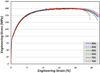 |
Fig. 1 Engineering stress–strain curves for uniaxial tensile tests of AA7075-O [23]. |
| In the text | |
|
Fig. 2 Setup of conducting in-plane cyclic loading experiments. |
| In the text | |
|
Fig. 3 Common ISF tool paths: left) Spiral (Helical) type tool path, right) Z-Level (Profile) type tool path. |
| In the text | |
|
Fig. 4 Effective strain distribution of sheet metal using different toolpath types. |
| In the text | |
|
Fig. 5 Tool reaction force by different toolpath types. |
| In the text | |
|
Fig. 6 Tool reaction moment by different toolpath types. |
| In the text | |
|
Fig. 7 Thickness-depth distribution for different toolpath types. |
| In the text | |
|
Fig. 8 Effective strain distribution of sheet metal using different step sizes. |
| In the text | |
|
Fig. 9 Tool reaction force by different step sizes. |
| In the text | |
|
Fig. 10 Tool reaction moment by different step sizes. |
| In the text | |
|
Fig. 11 Thickness-depth distribution for different step sizes. |
| In the text | |
|
Fig. 12 Effective strain distribution of sheet metal using different tool sizes. |
| In the text | |
|
Fig. 13 Tool reaction force by different tool sizes. |
| In the text | |
|
Fig. 14 Tool reaction moment by different tool sizes. |
| In the text | |
|
Fig. 15 Thickness-depth distribution for different tool sizes. |
| In the text | |
|
Fig. 16 Effective strain distribution of sheet metal using different feed rates. |
| In the text | |
|
Fig. 17 Tool reaction force by different feed rates. |
| In the text | |
|
Fig. 18 Tool reaction moment by different feed rates. |
| In the text | |
|
Fig. 19 Thickness-depth distribution for different feed rates. |
| In the text | |
|
Fig. 20 Effective strain distribution for different friction coefficients. |
| In the text | |
|
Fig. 21 Tool reaction force by different friction coefficients. |
| In the text | |
|
Fig. 22 Tool reaction moment by different friction coefficients. |
| In the text | |
|
Fig. 23 Thickness-depth distribution for different friction coefficients. |
| In the text | |
|
Fig. 24 Effective strain distribution of sheet metal using different wall angles. |
| In the text | |
|
Fig. 25 Tool reaction force by different wall angles. |
| In the text | |
|
Fig. 26 Tool reaction moment by different wall angles. |
| In the text | |
|
Fig. 27 Thickness-depth distribution for different wall angles. |
| In the text | |
|
Fig. 28 TCT stress–strain curve experiment vs. extended Voce, Chaboche with one back-stress term, and Chaboche with two back-stress terms. |
| In the text | |
|
Fig. 29 Effective strain distribution of sheet metal using different hardening models. |
| In the text | |
|
Fig. 30 Tool reaction force by different hardening models. |
| In the text | |
|
Fig. 31 Tool reaction moment by different hardening models. |
| In the text | |
|
Fig. 32 Thickness-depth distribution for different hardening models. |
| In the text | |
Current usage metrics show cumulative count of Article Views (full-text article views including HTML views, PDF and ePub downloads, according to the available data) and Abstracts Views on Vision4Press platform.
Data correspond to usage on the plateform after 2015. The current usage metrics is available 48-96 hours after online publication and is updated daily on week days.
Initial download of the metrics may take a while.