| Issue |
Mechanics & Industry
Volume 27, 2026
Artificial Intelligence in Mechanical Manufacturing: From Machine Learning to Generative Pre-trained Transformer
|
|
|---|---|---|
| Article Number | 19 | |
| Number of page(s) | 15 | |
| DOI | https://doi.org/10.1051/meca/2026011 | |
| Published online | 24 April 2026 | |
Original Article
Mechanical characteristic failure analysis and intelligent diagnosis method of filter bank circuit breakers in UHVDC projects
1
Electric Power Research Institute, State Grid Sichuan Electric Power Company, Chengdu 610048, Sichuan, PR China
2
State Grid Southwest Electric Power Research Institute CO. LTD, Chengdu 610042, PR China
3
State Grid Sichuan Electric Power Company, Chengdu 610042, Sichuan, PR China
* e-mail: This email address is being protected from spambots. You need JavaScript enabled to view it.
Received:
31
October
2025
Accepted:
25
February
2026
Abstract
In order to address the problem of mechanical degradation of filter group circuit breakers in UHVDC projects caused by the coupling of multiple factors such as mechanism jamming, lubrication failure, and micro-deformation of connecting rods, existing monitoring methods rely on single electrical features, making it difficult to effectively identify and decouple complex fault sources, seriously restricting equipment status perception and predictive maintenance capabilities. To this end, this paper proposes an intelligent diagnosis method that integrates multi-physics field mechanism modeling and multi-source heterogeneous sensing. First, an electromagnetic-mechanical-contact multi-field coupling simulation model is constructed to identify key observable features sensitive to various types of degradation. Second, four types of signals, namely operating current, vibration, acoustics, and displacement, are synchronously collected in a strong electromagnetic interference environment, and high-dimensional heterogeneous features are extracted by combining time-frequency analysis and graph convolutional networks. Finally, a multimodal fusion architecture based on a dual-branch attention mechanism is designed to achieve dynamic weighting and precise decoupling of complex degradation sources. Experimental results show that the method achieves a macro-average F1-score of 96.3% under 13 operating conditions and a triple-combination fault decoupling success rate of 89.3%. It also demonstrates excellent robustness in small sample sizes, noise interference, and historical field case backtesting. This method is beneficial to improving the state perception accuracy and fault warning capabilities of key switchgear in UHV converter stations. The research results provide strong technical support for building a safe, reliable, and intelligent new power system and have important engineering application value and social benefits.
Key words: Circuit breaker mechanical fault diagnosis / multi-physics coupling modeling / multi-modal sensor fusion / composite fault decoupling / graph neural network for condition monitoring
© J. Wang et al., Published by EDP Sciences 2026
 This is an Open Access article distributed under the terms of the Creative Commons Attribution License (https://creativecommons.org/licenses/by/4.0), which permits unrestricted use, distribution, and reproduction in any medium, provided the original work is properly cited.
1 Introduction
With the advancement of the “dual carbon” goals and the deepening implementation of the West-to-East Power Transmission Strategy, ultra-high voltage direct current (UHVDC) transmission projects have become a core component of my country’s new power system backbone network [1–3]. As key reactive power and harmonic control equipment in converter stations, AC filter banks need to be frequently switched on and off to dynamically balance the system’s reactive power demand, and their supporting circuit breakers can operate hundreds of times annually [4–6]. Under these high-load and high-reliability requirements, the circuit breaker mechanical system is subjected to complex stresses for a long time, is prone to performance degradation and even sudden failure, and seriously threatens the safe and stable operation of the DC system [7–9]. However, current circuit breaker status monitoring still relies mainly on regular maintenance and simple electrical parameter recording, which makes it difficult to timely detect early signs of mechanical degradation, exposing prominent problems such as weak status perception capabilities and delayed fault warning.
This paper focuses on the mechanical characteristic failure problem of dedicated circuit breakers for filter groups in UHVDC projects. Due to the frequent switching of capacitive loads, the operating mechanism of this type of circuit breaker is in a high dynamic stress state for a long time. Typical degradation modes such as transmission mechanism jamming, lubrication failure, and connecting rod micro-deformation often do not occur in isolation but present multi-factor coupling and gradual evolution characteristics. This type of composite degradation not only leads to macroscopic performance anomalies such as opening and closing time drift and contact speed reduction but is also likely to induce serious faults such as heavy breakdown and refusal to operate. In recent years, many scholars have conducted in-depth research on this subject: Park et al. proposed a resistive mechanical DC circuit breaker with resistive superconducting elements, which is a combined model of resistive superconducting elements and mechanical DC circuit breakers. It limits the initial fault current by quenching the resistive superconducting element [10]. Liu et al. developed an accurate finite element model of a lightning arrester to study the electrothermal and mechanical stresses during DC current interruption [11]. Yousaf et al. used feature extraction tools such as fixed wavelet transform and artificial neural networks based on random search to detect transmission line faults in a DC network. The goal is to improve the accuracy and reliability of protection relays due to various fault events [12]; Ma et al. verified that spring fatigue is exponentially related to the extension of tripping time through accelerated aging experiments [13]; and Wadie proposed a solution, namely the universal high voltage cloud battery (UHVCB, suitable for HVDC transmission and HVAC systems) universal high voltage cloud electricity concept design. Such a concept makes the production of CB (circuit breaker) faster, easier, and more economical per unit cost [14]. The above work together shows that the mechanical system of the filter bank circuit breaker is a vulnerable link under the coupling of multiple physical fields and multiple factors, and it is urgent to establish an accurate diagnosis system for complex degradation.
Existing research on circuit breaker mechanical fault diagnosis primarily relies on single electrical features, such as the operating coil current waveform or the opening and closing time, and uses threshold discrimination or shallow models such as support vector machines (SVMs) for state classification [15,16]. In recent years, some researchers have attempted to introduce vibration or acoustic signals and use convolutional neural networks (CNNs) or long short-term memory networks (LSTMs) for time series modeling [17,18]. However, existing methods generally have two major limitations: firstly, they rely only on a single electrical feature or simply concatenate multimodal data, failing to deeply integrate the multiphysics coupling mechanism of the device, resulting in insufficient interpretability of feature physics [19–21]. Secondly, there is a lack of effective modeling of the inherent correlation between multi-source signals, which makes it difficult to achieve precise decoupling and primary/secondary discrimination of fault sources when facing complex degradation scenarios with multiple coupled factors such as jamming, lubrication failure, and micro-deformation of connecting rods [22,23]. In summary, the existing methods still have obvious shortcomings in mechanism fusion depth, multimodal collaboration capability, and composite fault decoupling accuracy.
To overcome these bottlenecks, this paper aims to construct a dual-mechanism and data-driven intelligent diagnostic framework to accurately decouple and locate the sources of complex mechanical degradation in filter bank circuit breakers. Specifically, a multi-physics coupled failure model of the circuit breaker’s mechanical system is established based on multibody dynamics and electromagnetic theory to screen for key observable features sensitive to different degradation conditions. Four heterogeneous signals—operating current, housing vibration, partial discharge acoustics, and contact displacement—are then simultaneously collected. Time-frequency analysis and a graph neural network (GNN) are then combined to extract highdimensional discriminative features. Finally, a multimodal fusion diagnostic architecture based on an attention mechanism is designed to dynamically weight the contributions of each modality to achieve fine-grained identification of complex faults.
This method, for the first time, deeply integrates circuit breaker mechanical degradation mechanism modeling with multi-source heterogeneous sensing, overcoming the blind spots of traditional single-feature diagnosis in complex fault scenarios. By constructing a closed-loop diagnostic path of “physical guidance, data drive, and intelligent fusion”, it not only improves fault decoupling capabilities and diagnostic interpretability but also provides a scalable technical paradigm for condition-based maintenance of critical UHV switchgear, demonstrating significant theoretical innovation and promising engineering applications.
2 Intelligent diagnosis method of mechanical characteristics of circuit breakers by integrating multi-source sensing and mechanism driving
2.1 Multi-physics coupling failure mechanism modeling and sensitive feature screening
In order to accurately characterize the mechanical behavior of the filter bank circuit breaker under complex degradation conditions, a multi-physics field coupling simulation model covering electromagnetic drive, mechanical transmission, and contact dynamics is constructed, as shown in Figure 1.
This model reproduces the geometric structure of a 550 kV SF (sulfur hexafluoride) circuit breaker operating mechanism at a 1:1 scale, including key components such as the opening and closing coils, energy storage springs, transmission linkage, crank arm, and contact system. Material properties were set based on actual engineering parameters; among them, the material parameters of key components are sourced from the manufacturer’s technical manual and measured data: the operating mechanism housing is made of cast steel with an elastic modulus of 210 GPa and a density of 7850 kg/m3. The transmission connecting rod is made of high-strength alloy steel with an elastic modulus of 190 GPa and a density of 7800 kg/m3. The spring material is silicon chromium steel with an elastic modulus of 206 GPa. These parameters are consistent with the actual engineering materials of the 550 kV SF6 circuit breaker, and the baseline friction coefficient of the guide rail sliding pair was set to 0.05.
During the modeling process, the electromagnetic module calculates the driving force generated by the coil after it is energized based on the Maxwell equations [24], taking into account the core saturation effect and eddy current loss; the mechanical transmission module adopts the rigid-flexible coupling multi-body dynamics method to perform modal reduction processing on key flexible components to balance computational efficiency and accuracy; The modal reduction processing adopts the Craig Bampton substructure modal synthesis method, which combines the degrees of freedom of the flexible component interface with the fixed interface main mode and can significantly reduce the system degrees of freedom while ensuring computational accuracy. In this model, the first 10 fixed interface modes are retained for key flexible components such as transmission links and operating rods, with modal truncation frequencies covering the range of 0−2000 Hz, covering the main excitation frequency bands during the mechanism’s action process; the contact dynamics module introduces the Hertz contact theory and Coulomb friction model to describe the collision and sliding behavior during the contact closing/separation process [25,26].
For the three typical degradation modes commonly seen in engineering, controllable disturbances are applied to the model, respectively:
Mechanism jamming: By increasing the friction coefficient of the guide rail sliding pair to 0.12−0.18, the increased motion resistance caused by foreign matter intrusion or surface corrosion is simulated;
Lubrication failure: Increasing the rotational damping coefficient at the rotary hinge by 30%−50% effectively reflects the increased energy dissipation caused by grease drying or loss;
Connecting rod micro-deformation: An initial bending displacement of 0.5−1.2 mm is applied to the main transmission connecting rod to simulate the plastic deformation under long-term stress cycles.
Based on this, 13 typical operating condition combinations (including normal state, jamming + lubrication failure, connecting rod deformation + jamming, and triple-combination degradation) were designed, and transient co-simulations were conducted. Fifty Monte Carlo simulations were run for each operating condition to account for parameter fluctuations. Output included time-series data such as coil current, contact displacement, velocity, mechanism acceleration, and contact force. Based on this data, eight observable indicators were extracted: opening time, closing time, average contact velocity, peak velocity, RMS (root mean square) energy of the vibration signal, current rise time, current inflection point, and dominant vibration frequency (using fast Fourier transform (FFT) to identify the maximum amplitude frequency among the first three dominant frequencies).
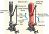 |
Fig. 1 Schematic diagram of the multi-physics coupling simulation model structure and degradation introduction position. |
2.2 Synchronous acquisition and preprocessing of multi-source heterogeneous signals
To acquire high-fidelity, highly synchronized, multi-dimensional status signals in the strong electromagnetic interference environment of a real-world UHV converter station, a four-channel, fiber-optically isolated, synchronous acquisition system was deployed. The system uses the opening/closing commands from the circuit breaker’s local control loop as an external trigger source and incorporates the GPS-PPS (global positioning system-pulse per second) signal as a global time reference, achieving nanosecond-level time synchronization and ensuring alignment of sensor data within microsecond accuracy. While the GPS-PPS provides a precise global time reference, its signal may be attenuated or unavailable in fully enclosed or deep indoor substation environments. To mitigate this risk, the system is designed with a backup synchronization mechanism. A high-stability local oscillator serves as a secondary time base, and its clock is disciplined by the GPS-PPS signal when available. In case of GPS signal loss, the system seamlessly switches to the disciplined local oscillator, maintaining synchronization accuracy sufficient for the diagnostic task. This dual-source design ensures reliable operation across varied field conditions. The four sensor types were deployed as follows.
Operating current i (t): A high-precision Hall current sensor is used, which is connected in series with the opening and closing coil circuit. Shell vibration a (t): IEPE (Integrated Electronics Piezoelectric) type accelerometers are installed at key positions of the operating mechanism box. Acoustic signal s (t) : An ultrasonic sensor with a center frequency of 40 kHz is used, which is mounted in the area near the sound source of the mechanism box to capture high-frequency acoustic emissions generated by mechanical impact, structural looseness, or abnormal friction. Linear displacement x (t): The contact movement stroke is measured non-contact by a laser displacement sensor. All analog signals are converted into optical signals for transmission through the optical fiber isolation module, completely cutting off the ground loop interference. The fiber optic isolation module model used is Analog Devices ADuM4160, with a common mode rejection ratio greater than 100 dB at 1 MHz and an isolation voltage of 5 kV RMS. The delay introduced by this module at a sampling rate of 50 kHz is less than 10 ns , ensuring high-fidelity transmission and microsecond-level synchronization accuracy of the signal in strong electromagnetic interference environments and effectively suppressing the common mode noise caused by switch operation, harmonics, and lightning in the converter station. The acquisition card uses a 16-bit ADC (analog-to-digital converter) with a uniform sampling rate of 50 kS/s to ensure that the Nyquist criterion is met and the transient details of the signal are retained [27].
Raw data preprocessing is a two-step process. Firstly, the four signals are subjected to five layers of wavelet decomposition using the db4 (Daubechies 4) wavelet basis. Based on the Stein unbiased likelihood estimation criterion, the threshold is adaptively determined to implement soft thresholding denoising while filtering out high-frequency electromagnetic noise and preserving key features such as action inflection points and shock pulses. Secondly, a sliding window of ±10 ms with the rising edge of the operation instruction as the reference time zero point is used to align the four-channel data in time, compensating for phase shifts caused by sensor response delays or differences in wiring length. The final output is a four-channel time-series dataset with uniform length, strict synchronization, and significantly improved signal-to-noise ratio, which serves as the standardized input for subsequent feature extraction modules. This serves as the standardized input for the subsequent feature extraction module. This process ensures the integrity and consistency of multi-source signals in complex electromagnetic environments, laying the data foundation for high-dimensional heterogeneous feature fusion.
2.3 High-dimensional feature extraction based on time-frequency-graph structure combination
Based on the four-channel synchronous timing signals i(t), a(t), s(t), and x(t) output in Section 2.2, differentiated feature extraction strategies are adopted for the physical characteristics of the signals to characterize the dynamic responses under different degradation mechanisms.
For the operating current i(t) and linear displacement x(t) signals, since they primarily reflect the timing characteristics of the overall mechanism motion, time-domain discriminant features are directly extracted: these include the opening/closing action time, current rise time, current inflection point, displacement curve inflection point location, contact average velocity, and maximum slope of the velocity curve. The velocity signal is obtained by performing a five-point smooth differential on the displacement signal x(t) to suppress the influence of numerical noise on the derivative calculation.
For the shell vibration a(t) and acoustic signal s(t), since they contain rich transient impact and frequency variation information, a time-frequency joint analysis method is used to extract high-dimensional features. First, the signal is subjected to a short-time Fourier transform (STFT) [28], with a window length of 1024 points and an overlap rate of 75% to obtain a time–frequency spectrum. The window length of 1024 points at a sampling rate of 50 kHz corresponds to a 20.48 ms temporal window. This duration is long enough to capture the complete transient impulse response during the circuit breaker’s opening/closing operation, while providing a frequency resolution of approximately 48.8 Hz, which is adequate to resolve the dominant vibration modes within the 0−2000 Hz range identified by the mechanism model. The 75% overlap rate is selected to increase the temporal sampling density of the time-frequency representation, reducing the potential for missing brief transient events and smoothing the spectrogram, thereby improving the stability of the extracted spectral features. At the same time, a six-layer wavelet packet transform (WPT) [29] is performed using the db8 wavelet basis to calculate the energy proportion of each subband and further calculate the wavelet packet energy entropy to quantify the signal complexity. In addition, the analytical signal is subjected to a Hilbert transform, the marginal spectrum is extracted, and its peak frequency is located as a characterization indicator of the mechanism’s resonance characteristics.
Based on the extraction of single-modal features, a multi-source signal correlation graph is constructed to model cross-modal dependencies. The four types of sensors are defined as the four nodes of the graph, and the node features are initialized to the time-frequency or time-domain feature vectors extracted from each. The feature vector dimension d of each node is 30, including the following feature categories: for current and displacement signals, extract six-dimensional time-domain features (such as action time, current rise time, displacement curve inflection point position, etc.); For vibration and acoustic signals, extract 12-dimensional time-frequency features (such as short-time Fourier transform spectral peaks, wavelet packet energy entropy, Hilbert marginal spectral peak frequencies, etc.). In addition, each node also contains six-dimensional statistical features (mean, variance, peak factor, waveform factor, pulse factor, and margin factor). Therefore, the dimension of the node feature matrix X is 4 × 30. The edge weights are determined by calculating the mutual information (MI) between any two signals [30]. The mutual information is estimated non-parametrically using the K-nearest neighbor method (K = 5) to capture nonlinear correlations. The selection of K value as 5 is based on the results of multiple pre-experiments. We compared the impact of graph structures constructed under four settings of K = 3, 5, 7, and 10 on classification performance on the validation set. The results showed that when K = 5, the embedded features extracted by the graph neural network achieved the highest macro average F1 score on the validation set. A low K value can easily be affected by noise, leading to unstable mutual information estimation, while a high K value can smooth out local nonlinear dependencies between signals. Around K = 5, the model performance is insensitive to changes in the K value, and the F1 score fluctuates by less than 0.5% when the range of variation is within ±1. In the undirected weighted graph G = (V, E, X) constructed in this way, V is the node set, E is the edge set, and X ∈ R4 × d is the node feature matrix.
The graph is fed into a three-layer graph convolutional network (GCN) [31]. Each layer uses the ReLU (Rectified Linear Unit) activation function, with output dimensions of 64, 32, and 16, respectively. Through a message passing mechanism, each node aggregates its neighborhood information, ultimately generating a graph embedding vector hGNN ∈ R16 that fuses cross-modal context. This vector is concatenated with the time–frequency feature vectors extracted independently from each modality to form the input of the subsequent fusion diagnosis module, as shown in Figure 2.
Figure 2 illustrates the joint feature extraction architecture: the top shows the time-frequency representation of the four signal types after STFT/WPT processing and the manual feature extraction process, while the bottom shows the sensor correlation graph constructed based on mutual information and the GNN encoding process, fully demonstrating the feature abstraction process from “physical signal → graph structure → embedding vector”. This method effectively combines the discriminative properties of a single modality with the dynamic characteristics of the time-frequency domain. It also explicitly models the physical coupling relationship between multi-source signals through a graph structure, providing a high-dimensional heterogeneous feature foundation for complex fault decoupling.
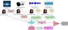 |
Fig 2 Architecture diagram of time–frequency-graph structure joint feature extraction. |
2.4 Multimodal fusion diagnosis model based on attention mechanism
Taking the heterogeneous feature vectors output in Section 2.3 as input, a dual-branch attention fusion diagnostic architecture is constructed to achieve decoupled identification of composite degradation sources. The input includes the time-frequency feature vectors of four modalities (current, vibration, acoustics, and displacement) and the cross-modal graph embedding vector hGNN ∈ R16 generated by the graph neural network. Each modal feature is first mapped to a unified dimension through an independent fully connected layer, forming a feature matrix F ∈ R5 × 64, where the five channels correspond to the four sensor signals and the graph embedding.
The fusion process adopts a dual-branch attention mechanism:
Channel attention branch: Global average pooling is performed on F along the modality dimension to obtain the channel statistical vector z∈R5, which is then passed through a two-layer fully connected network (intermediate dimension 8); the intermediate dimension was optimized and determined through grid search on the validation set. This article compared four configurations with intermediate dimensions of 4, 8, 16, and 32. Among them, dimension 8 achieved the highest macro average F1 score (95.1%) on the validation set with only 275k parameters, achieving the optimal balance between performance and lightweightness. When the dimension is 4, the model’s expressive ability is insufficient, and the F1 score drops to 92.3%; when the dimension is 16 or 32, the F1 scores are 95.0% and 95.2%, respectively, but the parameter count increases to 312k and 348k, which is not conducive to edge deployment); and a sigmoid activation function to generate channel weights wc ∈ [0, 1]5, which are used to adaptively weight the contribution of each modality to the diagnostic task [32].
Spatial attention branch: F is concatenated along the feature dimension and input into a one-dimensional convolutional layer (convolution kernel size 3, output channels 32). Then, a sigmoid function is used to generate time segment weights ws ∈ [0, 1]64, focusing on the key time region with the most information for fault identification. The weighted feature representation is:
 (1)
(1)
⨂ represents the outer product, and ⨀ represents the element-wise multiplication. Subsequently, Ffused is flattened and input into a three-layer fully connected classifier, while the output layer (activated with Softmax) generates probability distributions for 13 operating conditions (including normal and 12 single/composite degradation combinations). The tag system can recognize and prioritize multiple sources of degradation while supporting composite fault description.
To ensure the engineering practicality of the model, this study designed a lightweight architecture with a total number of parameters controlled at 275k. The training process used a cross-entropy loss function and Adam optimizer [33]. The dimensional changes and corresponding parameter consumption of each modality from the original signal to the fused features are recorded in Table 1, which demonstrates that the proposed architecture balances computational efficiency and edge deployment feasibility while maintaining strong discriminative ability.
Detailed breakdown of feature dimensions and model parameters by component.
3 Experimental setup
3.1 Experimental platform and sample construction
This study established a 1:1 scale testing platform for the mechanical characteristics of 550 kV SF6 filter bank circuit breakers, with the aim of verifying the effectiveness of the proposed method in a real physical environment. This platform fully reproduces the operating mechanism and simulated load of the arc extinguishing chamber. The simulated load of the arc extinguishing chamber is composed of a capacitive load unit and an inductive load unit connected in parallel, with an equivalent capacitance of 2500 pF and an equivalent inductance of 50 μH. It can reproduce the transient recovery voltage and current zerocrossing characteristics of the circuit breaker when opening and closing capacitive currents. The load is connected to the output terminal of the circuit breaker through a high-voltage cable, and during the opening and closing process, it generates electrical and thermal stresses similar to the switching of the filtering branch in actual engineering, ensuring that the mechanical stress borne by the mechanism is consistent with the on-site working conditions and standard control circuit in actual engineering, ensuring the engineering representativeness of experimental results. Its performance meets the requirements of the IEC (International Electrotechnical Commission) 62271-100 standard for mechanical operation testing.
The core of the platform lies in a set of precise adjustable degradation simulation devices, which are used to accurately reproduce three typical single degradation modes: (1) Mechanism jamming: By adjusting the preload of the guide rail slider, the sliding friction coefficient is gradually increased from the baseline value of 0.05 to 0.15 to simulate the increase in motion resistance caused by foreign matter intrusion or surface corrosion. (2) Lubrication failure: The amount of grease injected at the transmission arm hinge is quantitatively reduced to increase the rotational damping coefficient by 40%, which is equivalent to the increase in energy dissipation caused by grease drying or loss. (3) Connecting rod micro-deformation: To facilitate experimental reproduction and take into account the simulation coverage, the connecting rod micro-deformation is uniformly set to 0.8 mm, which is in the middle of the simulation setting range (0.5−1.2 mm) and is representative, in order to simulate the geometric deviation caused by material fatigue under long-term stress cycles. The selection of 0.8 mm as the experimental setting value is based on two reasons. Firstly, this value is at the median value set in the simulation, which can equally reflect the trend of the influence of the bending deformation on the mechanism dynamics when the upper and lower limits of the set interval change. Secondly, preliminary simulation analysis shows that within the range of 0.5−1.2 mm, key features such as displacement curve inflection point position, vibration frequency offset, and deformation are approximately linearly related. Therefore, the setting of 0.8 mm can effectively characterize the degradation effect within this linear interval without the need for experimental reproduction of all discrete values within the interval.
Based on the three types of single degradation described above, it further constructed pairwise and triple composite degradation scenarios, ultimately forming a structured dataset encompassing 13 operating conditions. This dataset covers normal conditions, three types of single faults, six types of dual composite faults, and three types of triple composite faults, fully encompassing the composite degradation scenarios likely to be encountered in engineering projects.
For each operating condition, 50 opening and closing operations were performed under strictly controlled environmental conditions (temperature 23 ± 2∘C and relative humidity <60%), with an interval of ≥60 s between each operation to prevent thermal accumulation from affecting the experimental results. The laboratory temperature was controlled to isolate the effects of mechanical degradation from environmental fluctuations. In a real converter station, ambient temperature can vary seasonally and diurnally, which may affect material properties (e.g., lubrication viscosity, spring stiffness) and sensor sensitivities. The proposed method addresses this through two aspects. First, the multi-physics simulation model incorporates temperature-dependent material properties, confirming that the key extracted features (e.g., timing, spectral peaks) remain predominantly sensitive to the targeted degradation modes rather than to slow thermal drifts. Second, the diagnostic model was tested on a supplementary dataset where the test platform temperature was varied between 5∘C and 40∘C. The macro-average F1-score degradation was less than 2.5%, demonstrating the method’s inherent robustness to typical operational temperature ranges.
All samples were randomly divided into training, validation, and test sets in a ratio of 7:2:1 to ensure a balanced distribution of various operating conditions across the subsets. To support subsequent decoupled diagnostic tasks, all samples in Table 2 were annotated using a composite label format, such as “Stick + Lubrication Failure (Primary: Stuck)”, clearly indicating the dominant and secondary degradation types.
Detailed list of 13 types of working condition samples.
3.2 Comparison methods and evaluation indicators
To fully verify the superiority of the proposed method in the decoupling diagnosis of composite faults, this paper selects two of the most representative advanced methods as the main comparison baselines, aiming to highlight the innovative value of this method from the two dimensions of multimodal fusion and end-to-end learning.
– SVM multi-feature fusion method: The manual features of three types of signals (current, vibration, and displacement) are fused (a total of 32 dimensions) to construct a high-dimensional feature vector and then input it into the SVM classifier. This method attempts to improve performance by simply splicing multimodal features but does not consider the inherent correlation between modalities.
– ResNet time series classification method: The four-channel original signal is directly spliced into a high-dimensional time series sequence and input into an 18-layer one-dimensional ResNet network [34] to achieve end-to-end fault mode learning. This method represents the current popular deep learning paradigm but ignores the guidance of physical mechanisms and multimodal collaboration.
All compared methods were trained and tested on the same experimental dataset—the 650 sets of samples described in Section 3.1 (split into training, validation, and test sets at a ratio of 7:2:1). To ensure a fair comparison, hyperparameters for all methods (such as the SVM penalty coefficient C, kernel function parameters, and ResNet learning rate) were optimized using grid search on the validation set.
The evaluation system uses three core indicators to comprehensively measure the performance of the model: (1) Accuracy (Accuracy, Acc): measures the proportion of correct classifications made by the model as a whole. (2) Macro F1-score (Macro F1): calculates the F1-score for each of the 13 categories and takes the arithmetic mean to evaluate the balanced performance of the model in each category, avoiding evaluation bias caused by category imbalance. (3) Composite fault decoupling success rate: This is the core evaluation indicator of this article. For the seven types of composite working conditions containing two or more degradation sources, if the prediction label output by the model can correctly identify ≥ 2 real dominant degradation types (e.g., the real label is “jamming + lubrication failure”, and the prediction result is “lubrication failure dominant + jamming secondary”), then the decoupling is judged to be successful. This indicator directly reflects the model’s ability to locate the root cause of complex faults.
Table 3 summarizes the key differences between the compared methods, providing a clear benchmark and reference for the performance comparison in Chapter 4.
Summary of performance benchmarks of comparison methods.
4 Results analysis
4.1 Analysis of the characterization capability of multi-source features for composite degradation modes
In order to quantify the ability of each modal feature to distinguish the composite degradation mode, single modal features (current, vibration, acoustics, and displacement) and multi-source fusion features were extracted, respectively, and the inter-class separability index was calculated on the test set. Linear Discriminant Analysis (LDA) was used to project the high-dimensional features into a two-dimensional space [35]. The mean Euclidean distance Dinter between the centers of each type of working condition and the mean intra-class covariance trace Dintra were calculated, and the separability index η = Dinter/Dintra was defined. The ratio η, known as the Fisher separability criterion or scatter ratio, is a standard metric in pattern recognition for evaluating the discriminative power of a feature set. It quantifies the ratio of between-class scatter to within-class scatter, where a higher value indicates better class separation in the feature space. This metric is widely used in fault diagnosis and condition monitoring literature to assess feature quality prior to classifier design. The larger the index, the higher the inter-class separation in the feature space, the stronger the intra-class clustering, and the better the potential performance of the diagnostic model.
Experimental results reveal the limitations of single modal features. As shown in Table 4, when using only the operating current signal, the separability index η is only 1.8, and the misjudgment rate for the two key combined operating conditions of “stuck + lubrication failure” and “stuck + connecting rod deformation” is as high as 42%. This indicates that while the current signal can reflect the overall electromagnetic-mechanical response, its single physical information makes it difficult to decouple the multiple coexisting degradation mechanisms. In contrast, when using vibration or acoustic signals alone, the η value increases to 2.5–2.7, and the misjudgment rate decreases, but it still cannot effectively distinguish between the “lubrication failure-dominated” and “stuck-dominated” combinations. The displacement signal is extremely sensitive to velocity but lacks response to high-frequency shocks, with an η value of 2.3.
This trend is clearly confirmed in Figure 3. Figure 3 shows the distribution of four representative feature schemes in the LDA two-dimensional projection space:
The distribution of four feature schemes in LDA two-dimensional space:
Current signal only (η = 1.8): The point cloud is highly overlapped, especially the red and purple triangles representing “stuck + lubrication failure (F4)” and “stuck + connecting rod deformation (F5)”, which are mixed together, confirming that a single current feature is difficult to decouple the complex fault.
Vibration signal only (η = 2.7): The categories begin to separate initially, but there is still an overlap between F4 and F5. This indicates that although a single vibration feature is better than current, it is still not enough to accurately distinguish friction-related composite faults.
Original four-modal fusion (η = 4.7): The clustering effect of each category is significantly improved, and F4 and F5 are basically separated, indicating that simple fusion can improve separability by utilizing multi-source information.
The complete method of this paper (η = 6.2): All 13 operating conditions (including F4 and F5) form clear, compact independent clusters with the largest inter-class spacing and the highest intra-class concentration, fully demonstrating the effectiveness of the “time-frequency-graph structure joint feature extraction” strategy proposed in Section 2.3. This strategy not only integrates multimodal information but also models the physical coupling relationship between sensors through graph neural networks, thereby achieving a deep decoupled representation of complex fault sources.
In particular, under the “stuck + lubrication failure” operating condition, the current inflection point time and the main vibration frequency exhibit a strongly coupled offset, while the acoustic signal energy entropy and displacement velocity slope selectively respond to lubrication and stuck, respectively. The combination of multi-source features enables decoupled characterization of fault sources. This result demonstrates that a single current feature, reflecting only the overall electromagnetic-mechanical response, is difficult to decouple from multiple sources of degradation. However, multi-source heterogeneous features, by complementary sensing of different physical processes, significantly improve the separability of compound faults, laying the foundation for subsequent high-precision diagnosis.
Separability index η of various feature combinations and typical compound fault misjudgment rate.
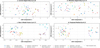 |
Fig. 3 Visualization of LDA dimensionality reduction under different feature combinations. |
4.2 Verification of the effectiveness of the multimodal fusion mechanism
To verify the ability of the multimodal fusion mechanism to mine cross-modal complementary information, four sets of ablation experiments were conducted:
Full Model: Complete architecture, including time-frequency feature extraction, GNN graph embedding, and dual-branch attention fusion;
w/o GNN: remove the graph neural network module and only use manually extracted time-frequency features for fusion;
w/o Attention: retain GNN, but turn off channel and spatial attention, and use simple splicing + fully connected fusion;
Late Fusion: Each modality trains a classifier independently and finally outputs the result through voting integration.
All variants were trained on the same training and test sets, using the macro-average F1-score as the primary evaluation metric to ensure balanced evaluation of the 13 operating conditions (especially the minority of complex fault classes). The experimental results are shown in Table 5.
The complete model achieved the highest F1-score of 96.3%. After removing GNN from the complete model, the overall performance significantly decreased to 89.7%, indicating that graph structure modeling effectively captured the nonlinear dependencies between sensors. After turning off the attention mechanism, the F1 score decreased to 91.2%, indicating that adaptive allocation of modal weights plays an irreplaceable role in suppressing redundant information and highlighting key discriminative features. The simplest late fusion strategy performed the worst (F1 = 85.4%), which strongly proves that early fusion at the feature level is far superior to later integration at the decision level, highlighting the design advantages of this architecture at the information fusion level.
This paper provides an in-depth analysis of the specific behavior of the attention mechanism under the typical composite working condition of “jamming + lubrication failure”, as shown in Figure 4, with the aim of further exploring the decision-making mechanism within the model.
Figure 4a shows that the channel attention mechanism assigns differentiated weights to different modalities: vibration (0.25) and displacement (0.22) signals receive the most attention, which is consistent with their dominant role in reflecting mechanical motion anomalies; the current signal has the lowest weight (0.14), which is consistent with the mechanism analysis due to its delayed response and lack of fault specificity; acoustic (0.18) and graph embedding (0.21) also obtained reasonable weights, reflecting the effective fusion of multi-source information.
The spatial attention in Figure 4b reveals the model’s focus on key periods during the opening cycle (0−100 ms): two significant peaks appear at 0−15 ms (mechanism start-up impact) and 45−60 ms (contact separation), which are highly consistent with the dynamic characteristics revealed by multiphysics simulation, indicating that the model can automatically lock in the most diagnostic time window.
In summary, GNN and the dual branch attention mechanism work together—GNN explicitly characterizes the physical relationships between sensors, while the attention mechanism dynamically highlights key modes and temporal segments. The combination of the two significantly enhances the ability to extract complementary and discriminative information from multi-source heterogeneous signals, providing core support for high-precision and interpretable composite fault decoupling diagnosis.
Comparison of ablation test performance.
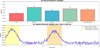 |
Fig 4 Attention weight distribution under the condition of jamming + lubrication failure. |
4.3 Evaluation of composite fault decoupling identification performance
This paper conducts fault source localization experiments on 7 types of composite fault conditions included in the test set, with the aim of quantitatively evaluating the method’s ability to decouple and identify multi-source degradation mechanisms. The labels for each type of working condition clearly indicate the dominant and secondary dominant degradation types (such as “jamming dominant + lubrication failure secondary”), and the model output is a 13-dimensional probability distribution, where the composite category corresponds to predefined decoupling labels.
Using the “success rate of decoupling composite faults” as the core indicator, it is defined as the proportion of samples in which the model correctly identifies ≥2 real degradation sources (with consistent primary and secondary relationships) in the composite fault samples. Simultaneously record individual recall rates for each type of degradation (jamming, lubrication failure, connecting rod deformation) to evaluate fine-grained positioning capability. The experimental results show that the method proposed in this paper exhibits excellent decoupling performance under various composite working conditions. The specific data is shown in Table 6.
According to Table 6, compared to the SVM fusion and ResNet baseline methods, our method has the highest decoupling success rate on all 7 types of composite faults. For example, the success rate of our method in the most challenging triple composite condition F7 (jamming + lubrication failure + connecting rod deformation) is 89.3%, while SVM and ResNet are only 63.0% and 48.5%, respectively. In addition, the method proposed in this paper generally has higher recall rates for various single degradation types, indicating that it cannot only identify composite patterns but also accurately locate the specific root cause of degradation.
To further explore the model’s classification performance on a global scale, Figure 5 verifies its ability to distinguish between easily confused categories.
Figure 5 shows the prediction accuracy of the model for 13 types of operating conditions on the test set. Normal state is 98.0%, and single jamming is 97.0%. For composite fault categories such as “jamming + lubrication failure (J)” (F4), the diagonal value is 94.0%, indicating that the model can accurately identify the composite mode.
Upon careful observation of all 9 types of composite faults circled by the purple dashed box in Figure 5, it can be observed that the values on non-diagonal lines are extremely small, mostly below 1.0, and the critical cross-misjudgment rates (such as between “connecting rod deformation + jamming” and “connecting rod deformation + lubrication failure”) are all below 3%. This low cross-validation rate is an important factor in achieving high-precision decoupling and localization of fault sources, and it strongly proves that the model can effectively distinguish the coupling characteristics between different types of friction degradation and structural deformation.
The real-time performance of the proposed model is evaluated through inference time. On an embedded industrial control platform equipped with an Intel Core i7-12700H processor and NVIDIA RTX 3060 graphics card, the average time required to complete the entire process from preprocessing and feature extraction to fault diagnosis of a single circuit breaker action 4-channel signal is about 45 milliseconds. The model has a parameter count of 275 k and occupies approximately 1.1 MB of memory. This inference time is much shorter than the minimum allowable interval time between two adjacent operations of the circuit breaker, meeting the real-time diagnostic requirements for monitoring the status of the converter station.
Details of the composite fault decoupling success rate and recall rate of each degradation type.
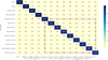 |
Fig. 5 Confusion matrix of degradation conditions of 13 types of circuit breakers. |
4.4 Small sample and noise robustness analysis
To evaluate the model’s applicability under real-world engineering constraints, it conducted small-sample training and noise-resistance testing. The experimental results, shown in Figure 6, demonstrate the robustness of the proposed method in data-scarce and high-noise environments.
In the small-sample experiment, 30% of the samples were randomly sampled from the original training set to retrain the proposed model and the comparison method, while all other settings remained unchanged. The original training set contains 455 samples, with 30% corresponding to approximately 136 samples. To ensure category balance, stratified random sampling was used to extract approximately 10 samples from each of the 13 working conditions, resulting in a small sample training set of 136 samples. The test results in Figure 6 show that the macro-average F1-score of the proposed method dropped from 96.3% to 91.8%, a decrease of 4.5 percentage points, while the SVM multi-feature fusion and ResNet performance dropped by 7.6 and 8.8 percentage points, respectively. This demonstrates that the proposed architecture maintains strong generalization capabilities under data-scarce conditions, attributed to the mechanism-guided feature design that reduces the reliance on large-scale annotated data. Figure 6a shows the macro-average F1-score trends of the three methods as the training sample ratio increases from 30% to 100%. As can be seen, the proposed method significantly outperforms the comparison method at all sample ratios, and its performance growth curve is more gradual, indicating that it is less dependent on data volume, and its advantage is particularly evident when data is limited.
In noise robustness experiments, Gaussian white noise was superimposed on all signal channels in the test set, with the signal-to-noise ratio (SNR) set to 20 dB to simulate strong electromagnetic interference environments on site. After noise contamination, the proposed method achieved an F1-score of 93.1%, a 3.2% performance degradation. SVM multi-feature fusion, due to its reliance on handcrafted features and its sensitivity to noise, saw its F1-score plummet by 7.2%. While ResNet, an end-to-end learning method, can automatically extract features, its generalization ability is limited under strong noise, resulting in an 8.2% F1-score drop. Figure 6b shows the F1-score degradation of the three methods at different SNRs (∞, 30, 20, and 10 dB). The proposed method maintained the highest performance at all noise levels, particularly at SNR = 20 dB, where its F1-score (93.1%) significantly exceeded that of the SVM fusion method (87.5%) and the ResNet method (85.3%).
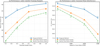 |
Fig. 6 Robustness comparison curve. |
4.5 Complex fault diagnosis backtracking and attribution analysis based on simulation cases
To validate the diagnostic accuracy and physical interpretability of this method under complex operating conditions, this section uses three typical filter bank circuit breaker failure events, reproduced using a precision degradation simulator on the experimental platform described in Section 3.1, as retrospective validation targets. These events are based on accurate simulations of common failure modes found in real-world projects (such as mechanism jamming, lubrication failure, and connecting rod deformation) to test the model’s ability to decouple degradation from multiple coupled factors.
At the time of the event, the synchronous data acquisition system had already recorded the operating current, mechanism vibration, and auxiliary contact signals at a sampling rate of 50 kS/s, covering the entire trip cycle. Following the preprocessing process described in Section 2.2, the raw recorded data was subjected to wavelet denoising and time alignment. The equivalent reconstruction of the displacement signal (estimated using a current-displacement mapping model) was supplemented; the current displacement mapping model is established based on the multiphysics field coupling simulation data in Section 2.1, and the nonlinear relationship between the operating current waveform and the displacement curve of the moving contact is fitted through Gaussian process regression. In the case retrospective, the current signal recorded onsite is input into the model to output displacement estimation values. The root mean square error between it and the actual displacement is calibrated in the laboratory to be less than 0.3 mm, which meets the diagnostic input accuracy requirements, based on the equipment inventory, forming a four-channel input.
The processed data is fed into the trained diagnostic model, which outputs a composite fault probability distribution. Figure 7 shows the diagnostic process for three simulation cases, demonstrating the model’s closed-loop capability from raw data to physical attribution.
Through in-depth analysis of Figure 7, it can draw the following conclusions:
For each test case, the model outputs a probability distribution over the 13 operating conditions via the final Softmax layer. The reported confidence level for a composite fault diagnosis is derived as the sum of the Softmax probabilities corresponding to all predefined composite labels that are consistent with the diagnosed primary and secondary degradation types. For instance, if the diagnosis is “jamming primarily, lubrication failure secondary”, the confidence is the sum of probabilities for the specific composite conditions (e.g., F4, F8) whose annotation matches this combination.
Case 1: Photos show guide rail corrosion, leading the model to diagnose it as “jamming primarily, lubrication failure secondary” (92.4% confidence level). The probability distribution plot shows the probabilities of the “jamming” and “lubrication” categories are 0.88 and 0.04, respectively, for a total of 0.92, highly consistent with the confidence level. More importantly, the signal waveforms in the center clearly demonstrate the distinct signatures of these two degradation modes in the current and vibration signals, providing solid data support for the model’s diagnosis. The 20 ms delay and 15% amplitude attenuation in the current waveform, along with the 0.45-fold energy attenuation and 0.8 kHz frequency shift in the vibration signal, are all quantitative indicators of this combined degradation.
Case 2: The photo focuses on the connecting rod joint, revealing visible bending deformation. The model diagnosed it as “connecting rod micro-deformation dominated” (89.7% confidence level), with a probability value of 0.89, accurately matching the confidence level. The signal waveforms in the center also show characteristic changes in the current and vibration signals caused by structural deformation, validating the validity of the model’s diagnosis. The rising slope of 0.02 A/ms in the current waveform and the low-frequency oscillation envelope of 0.5 Hz in the vibration waveform are key data features used by the model to identify this fault.
Case 3: Photos show signs of wear and dried grease at the hinge joint of the crank arm. The model diagnosed it as a combination of lubrication failure and jamming (90.1% confidence level). In the probability distribution plot, the “Lubrication” and “Jamming” categories show high probabilities of 0.85 and 0.05, respectively, for a total of 0.90, highly consistent with the confidence level. The signal waveform graph in the middle perfectly combines the characteristics of the first two cases, further demonstrating the model’s ability to accurately decouple combined faults. The current waveform’s 120 ms peak duration and 0.022 A/ms slope, along with the vibration signal’s 0.5× energy attenuation and 0.6 Hz low-frequency oscillation, together form the “data fingerprint” of this combined degradation.
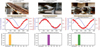 |
Fig. 7 Diagram of diagnostic results of three fault cases. |
5 Conclusion
This paper addresses the multi-factor coupled mechanical degradation problem of filter bank circuit breakers in UHVDC projects and proposes an intelligent diagnostic method that integrates multi-physics mechanism modeling and multi-source heterogeneous sensing. This method first constructs an electromagnetic-mechanical-contact multi-field coupled simulation model to screen key features sensitive to degradation factors such as sticking, lubrication failure, and connecting rod deformation. It then simultaneously collects current, vibration, acoustic, and displacement signals, extracting high-dimensional features through time-frequency analysis and graph neural networks. Finally, a dual-branch attention mechanism is used to achieve multimodal dynamic fusion and composite fault decoupling. Experiments demonstrate that this method achieves a macro-average F1 of 96.3% under 13 operating conditions and a triple composite fault decoupling success rate of 89.3%, significantly outperforming traditional single-feature or shallow fusion methods. The method also demonstrates good robustness and engineering applicability in small sample sizes, noise interference, and field retrospective verification. This study still has certain limitations: the degradation model constructed is based on three pre-defined typical faults and does not cover unknown or sudden fault types; The experimental verification was completed on a controlled laboratory platform, and although the on-site stress was simulated, it did not undergo long-term practical operation testing. Future work will focus on conducting long-term monitoring experiments on real converter stations and exploring unknown fault identification methods based on small samples and online learning.
Funding
This work was supported by Science and Technology Project of State Grid Sichuan Electric Power Company (Project No. 52199723003D).
Conflicts of interest
The authors have nothing to disclose.
Data availability statement
This article has no associated data generated and/or analyzed.
Author contribution statement
Conceptualization, J.W. and S.S.; Methodology, J.W.; Software, S.S.; Validation, J.W., S.S.; Formal Analysis, S.S.; Investigation, Z.L.; Resources, J.W.; Data Curation, J.W.; Writing—Original Draft Preparation, J.W., S.S.; Writing—Review & Editing, J.W.; Visualization, Z.L.; Supervision, Y.H., X.L.; Project Administration, D.Z., J.Z.; Funding Acquisition, J.W.
References
- R.P.P. Smeets, N.A. Belda, High-voltage direct current fault current interruption: a technology review, High Voltage 6, 171–192 (2021) [Google Scholar]
- K. Jacobs, S. Heinig, D. Johannesson et al., Comparative evaluation of voltage source converters with silicon carbide semiconductor devices for high-voltage direct current transmission, IEEE Trans. Power Electron. 36, 8887–8906 (2021) [Google Scholar]
- S. He, L. Hao, C. Liu et al., Master-slave control strategy of the cascaded multi-terminal ultra-high voltage direct current transmission system, IET Gener. Transm. Distrib. 17 3638–3647 (2023) [Google Scholar]
- C. Huang, E. Zhang, K. Guo et al., Potential application of Six Sigma method in operation and maintenance management of UHVDC converter station, Int. J. Emerg. Electr. Power Syst. 24, 151–162 (2023) [Google Scholar]
- H. Xiao, X. Duan, Y. Zhang, Accurate distinction of weak and strong AC grids for emerging hierarchical-infeed LCC-UHVDC systems, CSEE J. Power Energy Syst. 10, 772–777 (2023) [Google Scholar]
- Z. Guo, L. Hao, J. He et al., Complete protection strategy for loss of excitation in large-scale synchronous condensers applied to UHVDC transmission, CSEE J. Power Energy Syst. 11, 919–930 (2023) [Google Scholar]
- E. Taherzadeh, H. Radmanesh, S. Javadi et al., Circuit breakers in HVDC systems: state-of-the-art review and future trends, Prot. Control Mod. Power Syst. 8, 1–16 (2023) [Google Scholar]
- F. Mohammadi, K. Rouzbehi, M. Hajian et al., HVDC circuit breakers: a comprehensive review, IEEE Trans. Power Electron. 36, 13726–13739 (2021) [Google Scholar]
- F. Wadie, T. Eliyan, A universal high voltage SF6 circuit breaker for HVDC and HVAC systems, Sci. Rep. 15, 1200 (2025) [Google Scholar]
- S.Y. Park, H.S. Choi, Operation characteristics of a mechanical DC circuit breaker with a resistive superconducting element for high-reliability HVDC applications, IEEE Trans. Appl. Supercond. 33, 1–5 (2023) [Google Scholar]
- S. Liu, M. Popov, N.A. Belda et al., Thermal FEM analysis of surge arresters during HVDC current interruption validated by experiments, IEEE Trans. Power Deliv. 37, 1412–1422 (2021) [Google Scholar]
- M.Z. Yousaf, S. Mirsaeidi, S. Khalid et al., Multisegmented intelligent solution for MT-HVDC grid protection, Electronics 12, 1766 (2023) [Google Scholar]
- H. Ma, S. Zhou, C. Gao et al., Research on the reliability test and life assessment methods of relays used in circuit breaker operating mechanism, Energies 16, 4843 (2023) [Google Scholar]
- F. Wadie, T. Eliyan, Conceptional design for a universal HVDC-HVAC vacuum-interrupter-based circuit breaker, Sci. Rep. 14, 19816 (2024) [Google Scholar]
- J. Ruan, X. Wang, T. Zhou et al., Fault identification of high voltage circuit breaker trip mechanism based on PSR and SVM, IET Gener. Transm. Distrib. 17 1179–1189 (2023) [Google Scholar]
- X. Chen, H. Yuana, W. Niub et al., Mechanical fault diagnosis of high voltage circuit breaker based on acoustic vibration and IFPA-SVM, Int. Core J. Eng. 7, 98–104 (2021) [Google Scholar]
- S. Sun, S. Wei, J. Wang et al., Remaining useful life prediction for circuit breaker based on opening-related vibration signal and SA-CNN-GRU, IEEE Sens. J. 22, 23009–23022 (2022) [Google Scholar]
- S. Sun, Z. Wen, T. Du et al., Remaining life prediction of conventional low-voltage circuit breaker contact system based on effective vibration signal segment detection and MCCAE-LSTM, IEEE Sens. J. 21, 21862–21871 (2021) [Google Scholar]
- L. Ma, G. Wang, P. Zhang et al., Fault diagnosis method of circuit breaker based on CEEMDAN and PSO-GSA-SVM, IEEJ Trans. Electr. Electron. Eng., 17, 1598–1605 (2022) [Google Scholar]
- Y.A. Mohammed Alsumaidaee, C.T. Yaw, S.P. Koh et al., Detection of corona faults in switchgear by using 1D-CNN, LSTM, and 1D-CNN-LSTM methods, Sensors 23, 3108 (2023) [Google Scholar]
- Z. Xu, J. Yan, G. Sui et al., Intelligent mechanical fault diagnosis method for high-voltage circuit breakers based on Gray Wolf optimization and multi-grained cascade forest algorithms, Appl. Sci. 14, 3183 (2024) [Google Scholar]
- Y.A.M. Alsumaidaee, C.T. Yaw, S.P. Koh et al., Review of medium-voltage switchgear fault detection in a condition-based monitoring system by using deep learning, Energies 15, 6762 (2022) [Google Scholar]
- G. Sui, J. Yan, Y. Wu et al., Mechanical fault diagnosis of high-voltage circuit breakers with dynamic multi-attention graph convolutional networks based on adaptive graph construction, Appl. Sci. 14, 4036 (2024) [Google Scholar]
- DK. Durdiev, K.K. Turdiev, The problem of finding the kernels in the system of integro-differential maxwell, Appl. Ind. Math. 15, 190–211 (2021) [Google Scholar]
- G. Qinghua, Z. Xin, W. Zefeng et al., Calculation method of Hertz normal contact stiffness, J. Southwest Jiaotong Univ. 56, 883–888 (2021) [Google Scholar]
- Z. Liu, R.D. Howe, Beyond Coulomb: stochastic friction models for practical grasping and manipulation, IEEE Robot. Autom. Lett. 8, 5140–5147 (2023) [Google Scholar]
- A.R. Al Jabri, K.M. Abedin, S.M. Mujibur Rahman, The Nyquist criterion and its relevance in phase-stepping digital shearography: a quantitative study, J. Mod. Opt. 69, 804–810 (2022) [Google Scholar]
- Q. Zhang, L. Deng, An intelligent fault diagnosis method of rolling bearings based on short-time Fourier transform and convolutional neural network, J. Fail. Anal. Prev. 23, 795–811 (2023) [Google Scholar]
- D. Huang, W.A. Zhang, F. Guo et al., Wavelet packet decomposition-based multiscale CNN for fault diagnosis of wind turbine gearbox, IEEE Trans. Cybernetics 53, 443–453 (2021) [Google Scholar]
- H. Zhou, X. Wang, R. Zhu, Feature selection based on mutual information with correlation coefficient, Appl. Intell. 52, 5457–5474 (2022) [Google Scholar]
- U.A. Bhatti, H. Tang, G. Wu et al., Deep learning with graph convolutional networks: An overview and latest applications in computational intelligence, Int. J. Intell. Syst. 2023, 8342104 (2023) [Google Scholar]
- S. Kılıçarslan, K. Adem, M. Çelik, An overview of the activation functions used in deep learning algorithms, J. New Results Sci. 10, 75–88 (2021) [Google Scholar]
- M. Reyad, A.M. Sarhan, M. Arafa, A modified Adam algorithm for deep neural network optimization, Neural Comput. Appl. 35, 17095–17112 (2023) [Google Scholar]
- M. Chang, D. Yao, J. Yang, Intelligent fault diagnosis of rolling bearings using efficient and lightweight ResNet networks based on an attention mechanism (September 2022), IEEE Sensors J. 23, 9136–9145 (2023) [Google Scholar]
- S. Zhao, B. Zhang, J. Yang et al., Linear discriminant analysis, J. Nat. Rev. Methods Primers 4, 70 (2024) [Google Scholar]
Cite this article as: J. Wang, S. Sha, Z. Long, Y. He, X. Luo, D. Zhou, J. Zhang, Mechanical characteristic failure analysis and intelligent diagnosis method of filter bank circuit breakers in UHVDC projects, Mechanics & Industry 27, 19 (2026), https://doi.org/10.1051/meca/2026011
All Tables
Separability index η of various feature combinations and typical compound fault misjudgment rate.
Details of the composite fault decoupling success rate and recall rate of each degradation type.
All Figures
|
Fig. 1 Schematic diagram of the multi-physics coupling simulation model structure and degradation introduction position. |
| In the text | |
|
Fig 2 Architecture diagram of time–frequency-graph structure joint feature extraction. |
| In the text | |
|
Fig. 3 Visualization of LDA dimensionality reduction under different feature combinations. |
| In the text | |
|
Fig 4 Attention weight distribution under the condition of jamming + lubrication failure. |
| In the text | |
|
Fig. 5 Confusion matrix of degradation conditions of 13 types of circuit breakers. |
| In the text | |
|
Fig. 6 Robustness comparison curve. |
| In the text | |
|
Fig. 7 Diagram of diagnostic results of three fault cases. |
| In the text | |
Current usage metrics show cumulative count of Article Views (full-text article views including HTML views, PDF and ePub downloads, according to the available data) and Abstracts Views on Vision4Press platform.
Data correspond to usage on the plateform after 2015. The current usage metrics is available 48-96 hours after online publication and is updated daily on week days.
Initial download of the metrics may take a while.