| Issue |
Mechanics & Industry
Volume 26, 2025
|
|
|---|---|---|
| Article Number | 23 | |
| Number of page(s) | 18 | |
| DOI | https://doi.org/10.1051/meca/2025011 | |
| Published online | 23 July 2025 | |
Original Article
Analysis of the dynamic behavior of onboard rotors in non-linear regimes under the influence of parametric uncertainties
LMEst – Structural Mechanics Laboratory, Federal University of Uberlândia, School of Mechanical Engineering,
Av. João Naves de Ávila 2121,
Uberlândia,
MG
38408-100,
Brazil
* e-mail: This email address is being protected from spambots. You need JavaScript enabled to view it.
Received:
14
October
2024
Accepted:
25
March
2025
Abstract
In recent decades, a significant advance in the understanding of the dynamic behavior of rotors has been observed, including the capacity to model and forecast the physical behavior of these systems. The emergence of novel applications seeks to optimize performance and cost-effectiveness maintaining safe operating conditions and pushing rotating systems to their limits. Therefore, this contribution presents a combined numerical and experimental investigation of the nonlinear behavior exhibited by rotating systems subjected to base excitations. A comprehensive model incorporates nonlinear behavior resulting from large displacements as derived from the Lagrange’s equations and the finite element (FE) method. The deterministic model is extended to encompass bearings with stochastic stiffness. A rotating machine with a flexible shaft, a rigid disk, and supported by two bearings is evaluated. A dedicated test bench was used to compare the vibration responses obtained by using the implemented mathematical model with the experimental measurements. The obtained results demonstrate the representativeness of the considered FE model.
Key words: Rotordynamics / onboard rotors / finite element model / nonlinearities / parametric uncertainties
© T. R. B. Trevilato et al., Published by EDP Sciences, 2025
 This is an Open Access article distributed under the terms of the Creative Commons Attribution License (https://creativecommons.org/licenses/by/4.0), which permits unrestricted use, distribution, and reproduction in any medium, provided the original work is properly cited.
1 Introduction
Currently, there is a burgeoning global interest in optimizing industrial activities to make them more sustainable and environmentally friendly in response to significant climate changes, coupled with global demands for economically viable engineering projects while maintaining safety and comfort. This is further reinforced by the decreasing costs of renewable energy generation, that become economically viable as compared to fossil fuelbased energy generation [18]. This context has encouraged the improvement of the performance of rotating machines, and therefore current engineering rotors’ design should not only prioritize efficiency and reliability but also strive for self-sufficiency and sustainability whenever feasible.
The current industrial landscape also urges engineering disciplines to transcend traditional uses of rotors with well-established linear regimes and explore nonlinear ones. Fixed-base rotors experiencing linear operating regimes have been extensively investigated, and their dynamic behavior is well-documented [13]. However, a broad range of applications involve nonlinear rotors subjected to base excitations, such as aircraft engines. Nonetheless, the number of studies addressing this specific area is quite limited [4,5]. Research endeavors related to onboard rotors commonly focus on seismic excitations and excitations transmitted by the base from neighboring machinery and equipment, as claimed by Dakel et al. [8] and Al-Solihat et al. [1].
In more recent studies, Liu et al. [15] investigated the influence of base excitations on a rotor supported by hydrodynamic bearings. The FE model of the analyzed rotor is composed by a flexible shaft, a rigid disk, and two hydrodynamic bearings. The effects of the amplitude and excitation frequency of the base on the dynamic behavior of the rotor were investigated, and the authors demonstrated that the base velocity should not be disregarded when determining the bearing’s hydrodynamic forces. Furthermore, Del Claro et al. [9] evaluated two models for composite material onboard rotors: the first based on the Classical Beam Theory and the other is based on the Unified Theory. Three experimental test benches were employed to validate these methodologies, resulting a complete evaluation of the dynamic behavior of the rotor.
Regarding nonlinear effects affecting the dynamic behavior of rotors, Dakel et al. [7] delved into the nonlinear dynamic behavior of an onboard rotor supported by hydrodynamic bearings. The authors used a rotor FE model, which is able to incorporate various shafts and disks geometries (symmetrical or asymmetrical components). The considered model encompasses four degrees of freedom six types of base motion (three translations and three rotations) and accounts for the nonlinear characteristics of the oil film of the bearing. The Newmark integrator was employed to solve the time-dependent rotor equations of motion.
Lara-Molina et al. [14] conducted a sensitivity analysis of a flexible rotor affected by uncertain parameters, focusing on their effects on the rotor orbits and Campbell diagram. Barbosa et al. [2] carried out a sensitivity analysis of a flexible rotor made of composite material, as modeled by using the Simplified Homogenized Beam Theory [17].
In this context, the present contribution aims to investigate the nonlinear dynamic behavior of an onboard rotor affected by uncertainties in the bearing’s stiffness. A FE model of the rotor was formulated by considering the dynamic forces resulting from the base excitation applied to the onboard rotor [12]. In this case, nonlinearities are introduced in the rotor by considering that the transverse displacements of the shaft are no longer considered as being small (although still within the elastic material regime). The introduction of these nonlinearities and the solution of the resulting equations of motion follow the approach proposed by Zienkiewicz and Taylor [20]. The proposed model incorporates displacements in the transverse directions as well as rotations around these directions, which have yielded satisfactory results, as will be demonstrated later. Finally, uncertainties are included in the stiffness of the bearings, where the random field is discretized using the Karhunen-Loeve expansion method, thus generating uncertain envelopes for the results in the time domain.
It is worth mentioning that the novelty of the present contribution is the numerical and experimental investigations regarding the dynamic behavior of an onboard rotor in the existence of nonlinearities and uncertainties affecting the dynamic behavior of the system.
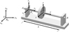 |
Fig. 1 Schematic representation of an onboard rotor. |
2 Mathematical model
This section presents the mathematical model of onboard rotors based on work of [10]. Part of the mathematical development is reproduced here, as it is relevant to the progression of this study and contributes to making the article more self-contained.
Taking the schematic representation of an onboard rotor shown in Figure 1 as a reference, wherein three reference axes are employed [10], R0(x0, y0, z0) denotes the inertial coordinate system, RS(xS, yS, zS) represents the mobile frame fixed to the rotor base and R(x, y, z) characterizes the mobile frame fixed to the disk.
The rotor orientations are described by using the Euler angles (Fig. 2) [13]. In this case, ψ, θ, and ϕ represent the motion of the reference R relative to the coordinate system RS, while α, β, and λ stand for the motion of RS relative to R0. Figure 2a represents the following reference rotations:
A rotation ψ around zS results in the intermediate reference frame R1 (x1, y1, z1);
A rotation θ around leads to another intermediate reference frame R2(x2, y2, z2);
A rotation ϕ is performed around y with y//y2.
Similarly, based on Figure 2b, the following can be deduced:
A rotation α around z0 results in the intermediate reference frame R3 (x3, y3, z3);
A rotation β around x3 leads to another intermediate reference frame R4 (x4, y4, z4);
A rotation λ is performed around y with y//y3.
Therefore, the angular velocity of R as described in the reference frame RS is expressed by equation (1). The angular velocity of RS as described in the reference frame R0 is represented by equation (2). The determination of the angular velocity of R (disk) as referenced in frame R0 (ground) is described as given by equation (3).
 (1)
(1)
 (2)
(2)
 (3)
(3)
where  denotes derivative with respect to time. The spatial position of the rotor base (vector
  ; Fig. 1) concerning the reference frame R0 is described by the coordinates xa, ya, and za, as given by equation (4). Conversely, the coordinates X, Y, and Z represent the position of this identical vector concerning the reference frame RS (Eq. (5)).
 (4)
(4)
 (5)
(5)
The position of the point C (vector  ; Fig. 1) with respect to the reference frame RS is presented by equation (6). Equation (7) presents the vector
  described in the reference frame RS.
 (6)
(6)
 (7)
(7)
herein u and w represent the transverse displacements of the shaft in RS along with the xS and zS axes, respectively. Additionally, y denotes the spatial coordinate of the disk along yS.
2.1 Kinetic energy
The kinetic energies of the symmetrical disk (TD), the unbalance mass (Tu), and the symmetrical shaft (TS) are provided by equations (8), (9), and (10), respectively.
 (8)
(8)
 (9)
(9)
 (10)
(10)
where Ix, Iy, and Iz are the area moments of inertia of the shaft associated with the axes x, y, and z, correspondingly. Meanwhile, mD is the mass of the disk, ρ denotes the material density, S is the cross-sectional area of the shaft, L is the shaft length, and mu represents the unbalance mass.
The translation velocity VC of the disk and the velocity VD of the unbalance mass, both relative to reference frame RS, are given by equations (11) and (12), respectively.
 (11)
(11)
 (12)
(12)
where t stands for the time and d represents the distance of the unbalance mass mu from the geometric center of the shaft at the position C and the point D represents the location of the unbalance mass, with the vector  relative to the reference frame RS given by:
 (13)
(13)
The mass moment of inertia tensor of the disk, denoted as ID (see Eq. (14)), comprises IDx, IDy, and IDz components, representing the mass moments of inertia associated with the x, y, and z directions, respectively.
 (14)
(14)
2.2 Strain energy
The strain energy U of the shaft remains constant along the motion of the rotor’s base [19]. This is associated to the fact that the deformation of the shaft results from the constraints imposed by the bearings. Therefore, for the formulation of the strain energy it is imperative to describe the shaft displacement field, as given by equation (15).
 (15)
(15)
where ue, ve, and we stand for the displacements in the x, y, and z directions, respectively, and u0 and w0 represent the displacements of the shaft mid-line along with the x and z directions, respectively.
Applying the displacement field to the Green-Lagrange strain tensor,
 (16)
(16)
in which ∇ is the gradient operator.
In scenarios characterized by small displacements the term 1/2 (∇u∇uT) can be neglected. However, in cases involving significant displacements, this term cannot be disregarded [12,20]. Thus, the strain field retaining the significant terms is given by:
 (17)
(17)
where {(),y = ∂ ()/∂y}.
Therefore, the strain energy of the system can be written as follows:
 (18)
(18)
where E and G are the Young and shear modulus, respectively.
2.3 Shaft FE model
The FE model of the shaft assumes a circular cross-section with constant diameter along the shaft length L, as presented in Figure 3. In this case, a beam theory is used to formulate a FE element with two nodes and four degrees of freedom each node: two displacements and two rotations (displacements u1, u2, w1, and w2; and rotations θ1, θ2, ψ1, and ψ2). The vector of nodal displacements for the shaft is given by equation (19).
 (19)
(19)
Consequently, the equations of motion representing the dynamic behavior of the rotor is written as:
 (20)
(20)
in which MD and DD represent the classical mass and gyroscopic matrices of the disk, respectively. The matrices ME and DE are the classic matrices of mass and gyroscopic of the shaft, respectively, while KE and Knl are the linear and nonlinear (representing the bending coupling between the xS and zS directions) stiffness matrices of the shaft, respectively. The matrices  , and
, and  are associated with the motion of the rotor base, as well as the force vectors
  and
and  . The matrices Kb and Db stand for the stiffness and damping due to the bearings, W represents the weight of the rotating components, and Fu is the unbalance forces. A comprehensive description of the mentioned FE matrices can be found in the “Appendix” of the present contribution.
2.4 Stochastic FE model
In the context of this study, the stiffness coefficients of the bearings were treated as uncertain parameters following a Gaussian random distribution [3,11]. To compute the associated stochastic stiffness matrices, the proposed model employs the Karhunen-Loève (KL) expansion method and the Latin Hypercube sampling to obtain a stochastic distribution of the mechanical properties. Given a stochastic process H(x, z, Θ),
 (21)
(21)
 (22)
(22)
where Θ is the variable associated to a realization (or sample) of the stochastic process, E [•] is the expectation operator, and C [•] stands for the covariance. Consequently, assuming that H(x, z, Θ) is a homogeneous Gaussian process with a symmetric and positive-definite covariance within the physical domain, the finite statistical approximation of this process of order m is expressed as follows [11]:
 (23)
(23)
where ξr (Θ) represents uncorrelated Gaussian variables. The terms λr = λiλj and fr (x, z) = fi (x) fj (y) correspond to the eigenvalues and eigenfunctions defined through the covariance function, respectively.
The eigenvalues and eigenfunctions are determined in terms of the roots wr of the following odd and even transcendental equations.
For odd i and j, with i ≥ 1 and j ≥ 1:
 (24)
(24)
with:
 (25)
(25)
Here, Lcor,x and Lcor,z represent the correlation lengths in the x and z directions within domains [−a, a] and [−a, a] where a and b denote the dimensions of the finite element used in the xS and zS directions, respectively. In the specific case of this work, both a and b are equal to the radius of the shaft.
The transcendental equations and the domain within which they are defined are obtained as follows:
 (26)
(26)
For i and j even, with i ≥ 2 and j ≥ 2:
 (27)
(27)
with:
 (28)
(28)
The transcendental equations and the domain in which they are defined are given by:
 (29)
(29)
The KL expansion has been employed for modeling the elementary random stiffness matrix of the bearings as given by:
 (30)
(30)
where  is the mean matrix calculated according to equation (20), while the stochastic matrix is defined as follows:
 (31)
(31)
in which kxx, kxz, kzx, and kzz are the stiffness coefficients of the bearings along the x and z directions.
3 Rotor test rig
Figure 4a shows the test rig used in the study of the onboard rotor. The rotor consists of a 550 mm long and 10 mm diameter flexible steel shaft (FE model composed of 21 beam elements; density ρ = 7800 kg/m3, Young’s modulus E = 190 GPa, and Poisson ratio v = 0.3), a rigid disk D (node 10, 2.3 kg mass) made of steel with 100 mm diameter and 40mm thickness (ρ = 7842 kg/m3), and two self-alignment ball bearings (B1 and B2, located at nodes 3 and 20, respectively). Displacement sensors (Meggitt TQ-412) were used to collect the rotor vibration responses at the disk position (orthogonally placed at node 10; sensors S10xs and S10zs). The system is driven by a DC electric motor. Measurements were taken using an Agilent® analyzer (model 35670A) with a range of 0 to 250 Hz in steps of 0.25 Hz. The rotational speed was controlled through a power source and verified by an encoder.
A model parameter updating procedure was performed to obtain the unknown parameters to be used in the FE model of the rotor, including the stiffness and damping coefficients of the bearings, the stiffness due to coupling between the electric motor and the shaft (Krotx and Krotz, around the orthogonal directions of the node 1), and the modal damping coefficients for the first two vibration modes.
The updating process was performed through the solution of a typical inverse problem based on simulated and experimental Frequency Response Functions (FRFs) of the rotor [6]. For this aim, the Differential Evolution optimization approach was applied [16].The objective function adopted in this case is presented by equation (32), in which only regions in the vicinity of the peaks associated with the natural frequencies were taken into consideration. The minimization of the objective function was carried out with an initial population of 100 individuals, and this process was repeated 10 times to determine the global minimum solution of the problem.
 (32)
(32)
where n is the number of FRFs used in the procedure, FRFexp represents the experimental data, and FRFnum corresponds to the numerical results obtained by the FE model of the rotating system.
The FRFs were acquired with the rotor at rest by applying impact forces along the xS and zS directions of the disk. The signal was measured by a proximity sensor positioned in the direction of the applied force, as shown in Figure 5, resulting two FRFs. Table 1 presents the parameters determined in the end of the optimization process, and Figure 5 illustrates the comparisons between the experimental FRFs and those obtained by the updated FE model. Note that the FE model is representative, particularly in the frequency range that encompasses the first two vibration modes of the rotor. The critical speeds of the rotor are approximately 1620 RPM (BW) and 1640 RPM (FW), as shown in the Campbell diagram presented in Figure 6.
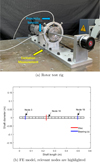 |
Fig. 4 Rotor test rig and FE model. |
4 Deterministic analyses
This section is dedicated to evaluating the dynamic behavior of the rotor under different base excitations.
In this case, the excitations were performed by using the Dongling Vibration® electrodynamic shaker (model GT1000) presented in Figure 7. In the conducted tests, the excitations were applied in the xS direction with the rotor operating at 1200 RPM (excitations measured by using an accelerometer).
Initially, the rotor was subjected to impacts with two different amplitudes: 1.5 m/s2 and 25 m/s2 within a 5 ms interval (Fig. 8). The associated numerical and experimental vibration responses of the rotor are presented in Figures 9 and 10, respectively. The vibration responses of the linear and nonlinear FE models are presented in Figures 9 and 10 for comparison purposes. Note that the 1.5 m/s2 excitation amplitude is insufficient to reveal the nonlinear existing in the rotor (see Fig. 9a). Consequently, the responses corresponding to the linear and nonlinear FE models were nearly identical. Furthermore, it can be concluded that the FE model adequately represents the dynamic behavior of the rotor in both directions for this excitation amplitude.
Figure 10 illustrates the vibration responses of the rotor obtained for a base excitation of 25 m/s2 amplitude. Note that the nonlinear effects became apparent, and the nonlinear FE model demonstrated to be more representative than the linear model. Figure 11 demonstrates the higher representativeness of the nonlinear model can be supported by the Discrete Fourier Transform (DFT) of the vibration responses, as presented in Figure 10. Note that the linear model is not able to represent satisfactorily the damped natural frequency of the rotor at, approximately, 1620 RPM (27 Hz). The unbalance response at 1200 RPM (20 Hz) is adequately represented by both linear and nonlinear FE models. The better response of the nonlinear model is primarily due to its better representation of stiffness increase, typical of nonlinearity of large displacements [20]. It is worth noting that, despite the displacements being smaller than the shaft diameter, It has already entered the large displacement regime, as evidenced by the responses.
Equation (33) presents the sinusoidal excitation applied along with the xS direction of the rotor.
 (33)
(33)
where Ωcr = 1560 RPM is a frequency close to the first BW and FW critical speeds of the rotor, n = 1/2 (or n = 1/3) is a constant used to produce submultiple excitations of Ωcr, and Γ defines the excitation amplitude (15 m/s2 and 30 m/s2 for n = 1/2 and n = 1/3, respectively). These values were determined based on the limitations of the electrodynamic shaker. Figure 12 presents the applied excitations.
Figure 13 illustrates the vibration responses of the rotor under the applied sinusoidal base excitations. Figures 13a and 13c demonstrate the ability of the nonlinear FE model to represent the dynamic behavior of the rotor in the direction that coincides with the direction of the applied excitation (xS direction). However, both linear and nonlinear models were not able to reproduce the experimental vibration responses of the rotor along the zS direction for n = 1/3 and n = 1/2 (see Figs. 13b and 13d). This difficult is associated with the model adopted to represent the coupling between the shaft and the electric motor. The linear stiffnesses Krotx and Krotz considered in the formulation are not representative enough in the context of the applied base excitation (see Fig. 12).
Figure 14 illustrates the numerical and experimental DFTs associated with the time domain vibration responses shown in Figure 13. Note that the nonlinear model was able to represent the experimental xS vibration responses of the rotor for the excitation frequencies corresponding to n = 1/3 and n = 1/2 and at Ωcr = 1560 RPM (see Figs. 14a and 14c, respectively). The lack of representativeness for both linear and nonlinear models regarding the experimental vibration responses of the rotor along the zS direction can be observed in Figures 14b and 14d, in which the higher differences between the numerical and experimental curves are observed in the frequency range 1400 to 2000 RPM. However, the nonlinear model can be considered as being better to describe the vibration responses of the rotor (see the performance of the nonlinear model at Ωcr = 1560 RPM in Fig. 14d).
The Mean Squared Errors (MSE values) of equation (34) considering the numerical and experimental vibration responses were determined for both linear and nonlinear cases for n = 1/2 and n = 1/3.
 (34)
(34)
where Nx represents the number of data points evaluated in the time interval 4s to 4.5 sec, ŷi denotes the experimental vibration amplitude and yi stands for the corresponding numerical responses determined by using either the linear or the nonlinear FE models. Table 2 presents the obtained MSE values and the corresponding standard deviations.
Table 2 reveals that for both cases (n = 1/3 and n = 1/2), the MSE values associated with the nonlinear model are smaller than the ones determined by using the linear model. For the case of n = 1/3, the errors of the nonlinear model are, approximately, 3.6 and 2 times smaller than those of the linear model for the xS and zS directions, respectively. In addition, considering n = 1/2, the errors of the nonlinear model were 2.6 and 1.8 times smaller than the errors of the linear model for the xS and zS directions, respectively.
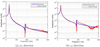 |
Fig. 5 Numerical and experimental FRFs of the rotor from node 10. |
Parameters obtained by the optimization procedure.
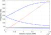 |
Fig. 6 Campbell diagram of the updated FE model. |
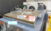 |
Fig. 7 Rotating system mounted on the electrodynamic shaker (control accelerometer used in the closed loop vibration control strategy of the shaker). |
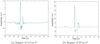 |
Fig. 8 Acceleration applied to the base of the rotor along the xS direction. |
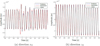 |
Fig. 9 Vibration response considering the 1.5 m/s2 impact excitation. |
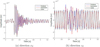 |
Fig. 10 Vibration response considering the 25 m/s2 impact excitation. |
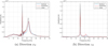 |
Fig. 11 DFTs of the impact response of 25 m/s2 amplitude. |
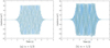 |
Fig. 12 Sinusoidal accelerations applied to the rotor base. |
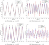 |
Fig. 13 Vibration responses of the rotor under sinusoidal base excitations. |
MSE values and standard deviations (Std.) determined considering the numerical and experimental vibration responses of the rotor.
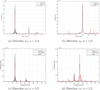 |
Fig. 14 Numerical and experimental DFTs associated with the vibration responses as presented in Figure 13. |
5 Stochastic analyses
However, it is necessary to ascertain whether the MSE values obtained using the nonlinear FE model (smaller MSE values) are statistically relevant. Hypothesis tests were performed for the four scenarios described in Table 2 (n = 1/2 and n = 1/3 for the xS and zS directions). The null hypothesis states that the MSE value of the linear model is smaller than or equal to the error obtained by using the nonlinear model, i.e., MSEL ≤ MSENL. Consequently, the alternative hypothesis is MSEL > MSENL. In all test cases, the null hypothesis is rejected in favor of the alternative hypothesis, accepted at a statistical significance level of, approximately, 15%. These results indicate that the nonlinear model leads to a significantly lower error than the linear model with statistical relevance.
Next, a stochastic model was introduced incorporating a 10% level of uncertainty in the bearing stiffness through the so-called Karhunen-Loève expansion (see Section 2.4) (refers to 10% chance in the standard deviation on the related Gaussian variables). In this case, an impulse with 25 m/s2 amplitude and a sinusoidal excitation considering n = 1/2 (see details in Eq. (33)) were applied to the rotor base, separately. A total of 200 samples were generated for the analysis of stochastic responses. For both cases the rotor operates at 1200 RPM. A convergence analysis was performed, by using mean square deviation, normalized by the average of all errors, as depicted in Figure 15, demonstrating that the convergence is achieved well before reaching 200 samples, but for greater robustness of the result, 200 samples were maintained.
Figure 16 presents the obtained uncertainty envelopes. As mentioned, only the vibration responses determined by using the nonlinear FE model are evaluated since it reveals to be more adapted to represent the experimental data (see Tab. 2). Concerning the impulse responses (Figs. 16a and 16b), it can be observed that the experimental vibration responses along the xS direction are included in the corresponding uncertainty envelopes. Additionally, the envelopes are narrower immediately after the impulse application and become wider as the signal is attenuated along the time. The uncertain envelopes are not able to represent the experimental vibration responses of the rotor measured along with the zS direction.
The envelopes associated with the sinusoidal excitation (see Figs. 16c and 16d) is narrower for the vibration responses obtained along with the force direction (xS direction). Additionally, note that the uncertain envelopes could represent better the vibration responses of the rotor along the xS direction as compared with the results obtained along the zS direction. It is also important to highlight that, despite the bearing stiffness being considerably lower than the shaft stiffness, the responses of the nonlinear system were particularly sensitive to uncertainties in this parameter.
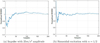 |
Fig. 15 Convergence analyses performed for both base excitation conditions. |
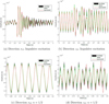 |
Fig. 16 Uncertain envelopes obtained by using the nonlinear FE model under two different excitation conditions. |
6 Conclusions
In the present study, a stochastic nonlinear onboard rotor FE model was formulated and experimentally validated. The dynamic analysis of the considered system demonstrates the considerable error margin associated with a linear model when nonlinearity due to large displacements should have been taken into account. In the direction of the applied excitatioArn (xS direction), the linear model overestimates the vibration response amplitude of the rotor. However, in the zS direction the linear model fails to capture the coupling of directions due to large displacements, resulting an underestimation of the actual vibration response amplitude. The linear model overestimates the sensitivity to the uncertainties applied to the bearing stiffness. The nonlinear model proposed in this study effectively represents the rotor responses along the xS direction and shows an improvement in the representation of the vibration responses along the zS direction as compared with the linear FE model.
It is worth mentioning that some model refinements are scheduled to be introduced in future work, such as the inclusion of shear effects and axial displacement. Finally,uncertainty analysis with respect to various parameters of the FE model by considering the rotor operating under different conditions is also scheduled.
Acknowledgements
The authors are thankful the Brazilian research agencies CNPq (Proc. Nb. 406148/2022-8), FAPEMIG (APQ-040034-24), and CAPES through the INCT-EIE for the financial support provided for this research effort. The authors also would like to thank the companies Foz do Chapecó, Baesa, Enercan and Ceran for technical and financial support, through the Research and Development project PD-02949-3007/2022 with fundings from ANEEL’s R&D program.
Funding
The Article Processing Charges for this article are taken in charge by the French Association of Mechanics (AFM).
Conflicts of interest
The authors declare that they have no conflict of interest.
Data availability statement
The data that support the findings of this study are available on request from the corresponding author, Dr. Aldemir Ap Cavallini Jr (This email address is being protected from spambots. You need JavaScript enabled to view it. ).
Author contribution statement
All authors participated and contributed to all parts, from the design and implementation of the research and experimental part, to the analysis of the results and to the writing of the manuscript. All authors agreed to the published version of the manuscript.
Ethical approval
Not applicable.
Appendix A Numerical integration
Equation (20) is numerically integrated by using a variant of the Newmark method. For this aim, the velocity  and acceleration
  vectors are given by [17]:
 (A.1)
(A.1)
where the subscript n indicates that the vector or matrix is calculated at time tn, and λ1 and λ2 are parameters of the Newmark method. Applying equation (A.1) to the equation of motion of the rotor (Eq. (20)), the following equation is obtained:
 (A.2)
(A.2)
where:

with:

Equation (A.2) is a system of nonlinear algebraic equations at the instant tn, which can be solved iteratively by using the Newton-Raphson method. This method is based on the expansion of the nonlinear algebraic equation into Taylor series around the known solution. In the formulation used in this work, it is assumed that to obtain the solution at iteration r, the solution at iteration r − 1 is known. Thus, a residual ϕ (qn) is defined:
 (A.3)
(A.3)
Expanding ϕ (qn) in Taylor series:
 (A.4)
(A.4)
where O q2 represents higher order terms. Using equation (A.3) and (A.4) and by considering the higher order terms as negligible:
 (A.5)
(A.5)
where tK is known as tangent matrix, or tangent stiffness matrix. The displacement increment can be given by:
 (A.6)
(A.6)
The calculation of the tK matrix is given by:
 (A.7)
(A.7)
which results in:
 (A.8)
(A.8)
where:

Appendix B Matrices and vectors of the equation of motion
The following matrices and vectors refer to Equation (20)
 (B.1)
(B.1)
 (B.2)
(B.2)
 (B.3)
(B.3)
 (B.4)
(B.4)
 (B.5)
(B.5)
where 
 (B.6)
(B.6)
 (B.7)
(B.7)
 (B.8)
(B.8)
 (B.9)
(B.9)
 (B.10)
 (B.11)
 (B.12)
 (B.13)
 (B.14)
 (B.15)
 (B.16)
 (B.17)
 (B.18)
References
- M.K. Al-Solihat, M. Nahon, K. Behdinan, Dynamic modeling and simulation of a spar floating offshore wind turbine with consideration of the rotor speed variations, J. Dyn. Syst. Meas. Control 141, 081014 (2019) [Google Scholar]
- P.C. Barbosa, V.T. Del Claro, M.S. Sousa, Jr., A.A. Cavalini, Jr., V. Steffen, Jr., Experimental analysis of the shbt approach for the dynamic modeling of a composite hollow shaft, Composite Struct. 236, 111892 (2020) [Google Scholar]
- M. Belonsi, A. de Lima, T. Trevilato, R. Borges, An efficient iterative model reduction method for stochastic systems having geometric nonlinearities, J. Braz. Soc. Mech. Sci. Eng. 42, 1–16 (2020) [CrossRef] [Google Scholar]
- Y. Briend, M. Dakel, E. Chatelet, M.A. Andrianoely, R. Dufour, S. Baudin, Effect of multi-frequency parametric excitations on the dynamics of on-board rotorbearing systems, Mech. Mach. Theory 145, 103660 (2020) [Google Scholar]
- Y. Briend, E. Chatelet, R. Dufour, M.-A. Andrianoely, F. Legrand, S. Baudin, Dynamics of on-board rotors on finite-length journal bearings subject to multi-axial and multi-frequency excitations: numerical and experimental investigations. Mech. Ind. 22 (2021) https://doi.org/10.1051/meca/2021034, DOI: 10.1051/meca/2021034 [Google Scholar]
- A. Cavalini, Jr., L. Sanches, N. Bachschmid, V. Steffen, Jr., Crack identification for rotating machines based on a nonlinear approach. Mech. Syst. Signal Process. 79, 72–85 (2016) [Google Scholar]
- M. Dakel, S. Baguet, R. Dufour, Bifurcation analysis of a non-linear on-board rotor-bearing system, in: International Design Engineering Technical Conferences and Computers and Information in Engineering Conference, American Society of Mechanical Engineers V008T11A060 (2014a) [Google Scholar]
- M. Dakel, S. Baguet, R. Dufour, Steady-state dynamic behavior of an on-board rotor under combined base motions, J. Vibr. Control 20, 2254–2287 (2014b) [Google Scholar]
- V.T. Del Claro, A.A. Cavalini, Jr., I.F. Santos, V. Steffen, Jr., On the modeling of flywheel rotor systems via unified formulation: Viability, practicalities, and experimental validation. Composite Struct. 299, 116030 (2022) [Google Scholar]
- M. Duchemin, A. Berlioz, G. Ferraris, Dynamic behavior and stability of a rotor under base excitation, ASME 128, 576 (2006) [Google Scholar]
- R.G. Ghanem, P.D. Spanos, Stochastic Finite Elements: A Spectral Approach, Courier Corporation (2003) [Google Scholar]
- M. Kapitaniak, V. Vaziri, M. Wiercigroch, Helical buckling of thin rods: Fe modelling, in: MATEC Web of Conferences, EDP Sciences, 02010 (2018) [Google Scholar]
- M. Lalanne, G. Ferraris, Rotordynamics Prediction in Engineering. John Wiley and Sons, Inc. (1998) [Google Scholar]
- F.A. Lara-Molina, A.A. Cavalini, Jr., E.H. Koroishi, V. Steffen, Jr., Sensitivity analysis of flexible rotor sub jected to interval uncertainties, Latin Am. J. Solids Struct. 16, 1–13 (2019) [Google Scholar]
- Z. Liu, Z. Liu, Y. Li, G. Zhang, Dynamics response of an onboard rotor supported on modified oil-film force considering base motion, Proc. Inst. Mech. Eng. Part C: J. Mech. Eng. Sci. 232, 245–259 (2018) [Google Scholar]
- K. Price, R.M. Storn, J.A. Lampinen, Differential Evolution: A Practical Approach to Global Optimization, Springer Science & Business Media (2006) [Google Scholar]
- J.N. Reddy, Mechanics of Laminated Composite Plates and Shells: Theory and Analysis. CRC Press (2003) [Google Scholar]
- M. Roser, Why did renewables become so cheap so fast. And what can we do to use this global opportunity for green growth 2 (2020) https://ourworldindata.org/cheap-renewables-growth [Google Scholar]
- M.S. Sousa, P.C. Barbosa, V.T.D. Claro, R. Nicoletti, A.A. Cavalini, V. Steffen, Numerical prediction and experimental validation of an onboard rotor under bending. Meccanica 56, 2631–2650 (2021) [Google Scholar]
- O.C. Zienkiewicz, R.L. Taylor, The Finite Element Method for Solid and Structural Mechanics. Elsevier (2005) [Google Scholar]
Cite this article as: Thales R. B. Trevilato, Aldemir Ap Cavallini Jr, Valder Steffen Jr, Analysis of the Dynamic Behavior of Onboard Rotors in Non-Linear Regimes Under the Influence of Parametric Uncertainties, Mechanics & Industry 26, 23 (2025), https://doi.org/10.1051/meca/2025011
All Tables
MSE values and standard deviations (Std.) determined considering the numerical and experimental vibration responses of the rotor.
All Figures
|
Fig. 1 Schematic representation of an onboard rotor. |
| In the text | |
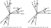 |
Fig. 2 Transformation of coordinates (Adapted from Lalanne and Ferraris [13]). |
| In the text | |
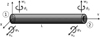 |
Fig. 3 Degrees of freedom associated with the finite element of the shaft [2]. |
| In the text | |
|
Fig. 4 Rotor test rig and FE model. |
| In the text | |
|
Fig. 5 Numerical and experimental FRFs of the rotor from node 10. |
| In the text | |
|
Fig. 6 Campbell diagram of the updated FE model. |
| In the text | |
|
Fig. 7 Rotating system mounted on the electrodynamic shaker (control accelerometer used in the closed loop vibration control strategy of the shaker). |
| In the text | |
|
Fig. 8 Acceleration applied to the base of the rotor along the xS direction. |
| In the text | |
|
Fig. 9 Vibration response considering the 1.5 m/s2 impact excitation. |
| In the text | |
|
Fig. 10 Vibration response considering the 25 m/s2 impact excitation. |
| In the text | |
|
Fig. 11 DFTs of the impact response of 25 m/s2 amplitude. |
| In the text | |
|
Fig. 12 Sinusoidal accelerations applied to the rotor base. |
| In the text | |
|
Fig. 13 Vibration responses of the rotor under sinusoidal base excitations. |
| In the text | |
|
Fig. 14 Numerical and experimental DFTs associated with the vibration responses as presented in Figure 13. |
| In the text | |
|
Fig. 15 Convergence analyses performed for both base excitation conditions. |
| In the text | |
|
Fig. 16 Uncertain envelopes obtained by using the nonlinear FE model under two different excitation conditions. |
| In the text | |
Current usage metrics show cumulative count of Article Views (full-text article views including HTML views, PDF and ePub downloads, according to the available data) and Abstracts Views on Vision4Press platform.
Data correspond to usage on the plateform after 2015. The current usage metrics is available 48-96 hours after online publication and is updated daily on week days.
Initial download of the metrics may take a while.