| Issue |
Mechanics & Industry
Volume 26, 2025
Recent advances in vibrations, noise, and their use for machine monitoring
|
|
|---|---|---|
| Article Number | 22 | |
| Number of page(s) | 19 | |
| DOI | https://doi.org/10.1051/meca/2025014 | |
| Published online | 01 July 2025 | |
Original Article
Verifying hyperparameter sensitivities of optimal filter design methods for fault signature enhancement
1
Centre for Asset Integrity Management, Department of Mechanical and Aeronautical Engineering, University of Pretoria,
Pretoria,
South Africa
2
School of Mechanical, Industrial & Aeronautical Engineering, University of the Witwatersrand,
Johannesburg,
South Africa
3
Department of Mechanical Engineering, KU Leuven,
Celestijnenlaan 300,
3001
Heverlee,
Belgium
4
Flanders Make @ KU Leuven,
Belgium
* e-mail: This email address is being protected from spambots. You need JavaScript enabled to view it.
Received:
7
March
2024
Accepted:
15
May
2025
Abstract
Optimal filters are designed in vibration-based condition monitoring to enhance weak fault signatures for improved diagnosis. While optimisation-based filter design approaches have matured, their validation has typically focused on final objective values and constraint satisfaction. However, ensuring robust and reliable results requires verifying the correctness of design sensitivities, i.e., the gradients of both objective and constraint functions with respect to design variables, as well as hyperparameter sensitivities. This paper emphasises the importance of confirming and quantifying a filter’s response to varying hyperparameters to ensure it meets design specifications. By rigorously verifying sensitivities, engineers can more confidently deploy optimal filter designs that enhance fault-related features, resulting in more effective fault detection and diagnosis in complex engineering systems.
Key words: Optimal digital filter design / gearbox fault detection / squared envelope spectrum / gradient-based optimisation
© S. Schmidt et al., Published by EDP Sciences, 2025
 This is an Open Access article distributed under the terms of the Creative Commons Attribution License (https://creativecommons.org/licenses/by/4.0), which permits unrestricted use, distribution, and reproduction in any medium, provided the original work is properly cited.
1 Introduction
In vibration-based condition monitoring of rotating machinery, weak fault signatures can be enhanced using digital filtering methods [1-3], which enable early fault detection, fault component identification and fault trending [4]. Filter design methods used in vibration-based condition monitoring include informative frequency band identification methods [3], blind deconvolution [1], blind filtering [5], wavelet filtering [6], sparse filtering [7], empirical mode decomposition [8], Wiener filtering [9], cyclic Wiener filtering [10], and adaptive filtering [11]. Machine learning models enable the realisation of more complex filter structures (e.g., convolutional sparse filtering [12]), by utilising historical data to extract important information from data [12-14].
Furthermore, in implementing these methods, decisions such as formulating objectives and choosing optimisation strategies must be critically validated [1,15]. To achieve this, validation involves verifying that (i) the objective function is correctly implemented, (ii) derivatives (if applicable) are accurate, (iii) the optimisation process itself does not distort performance, and (iv) parameter changes lead to expected and consistent changes in performance. Such rigorous evaluation confirms the method’s correctness and ensures its sensitivities reflect realistic behaviour, enabling robust comparisons with existing techniques and reliable conclusions in diverse applications. It is often possible to verify (i) using cases where the function value is easily estimated, and (ii) through numerical sensitivities like finite differences. Sensitivity analyses of optimal filtering hyperparameters are frequently performed (e.g., [16-19]) to assess the impact of hyperparameter choices. However, (iii) and (iv) are rarely explicitly addressed in the literature, despite likely being performed in published works.
To address this gap, a hyperparameter sensitivity verification framework is proposed and presented in Figure 1. The hyperparameter sensitivity verification framework involves interconnected optimal filtering and sensitivity analysis decisions. The general optimal filtering process is a structured approach for designing and evaluating filters. The optimal filtering hyperparameters, which affect the filter’s performance, must be set throughout the process. Sensitivity analysis is conducted to understand the impact of hyperparameter choices on the performance of the filter.
This involves selecting the hyperparameter sensitivity set, the sensitivity analysis approach, perturbation directions and step sizes. The sensitivities are subsequently computed and interpreted to determine how hyperparameter changes affect the system’s overall performance. Verification ensures that the sensitivity expectations align with the observed results, providing insights into the reliability of the filtering process.
The proposed hyperparameter sensitivity verification framework is applied to the established Indicator of second-order CycloStationarity (ICS2) objective (used in Maximum second-order CYClostationarity Blind Deconvolution (CYCBD) [16] and related methods [20,21]), and the recently proposed Generalised Envelope-based Signal-to-Noise ratio (GES2N) [15]. Rather than providing specific recommendations for parameter choices, which are highly dataset- and algorithm-dependent, or conducting a full-scale sensitivity analysis as advocated by Saltelli et al. [22], this work focuses on confirming expected trends when conducting hyperparameter studies as a first verification step of hyperparameter sensitivities. In summary, the contributions of the work are as follows:
A general sensitivity analysis strategy for hyperparameter sensitivity verification of optimal filter design is proposed.
A hyperparameter sensitivity verification study of the ICS2 (an established filter coefficient estimation objective) and the GES2N (a recently proposed objective for filter coefficient estimation) is performed for signals acquired under time-varying speed conditions.
The work is structured as follows: Section 2 presents an overview of the optimal filtering process and its hyperparameters. Subsequently, the hyperparameter sensitivity verification process for optimal filtering is presented in Section 3. The hyperparameter sensitivity verification of the ICS2 and GES2N objectives are presented in Section 4 and the study outline in Section 5. The results are presented in Section 6, whereafter the work is concluded in Section 7.
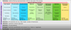 |
Fig. 1 This conceptual framework illustrates an optimal filtering workflow, starting with raw input signals and progressing through pre-processing, transformations, objective definition, and optimisation towards performance evaluation. On the left, various methods of preparing and transforming signals are shown, while the centre section focuses on formulating the optimisation problem and selecting suitable optimisation algorithms. Performance metrics and approaches for evaluating filter quality are presented on the right. Below, a HyperParameter (HP) sensitivity verification strategy ensures robust and verified filter designs. Abbreviations: AR: Auto-Regressive, CG: Congjugate Gradient, HT: Hilbert Transform, ICS2: Indicator of second-order CycloStationarity, QN: Quasi-Newton, RMSE: Root-Mean-Squared Error, SES: Squared Envelope Spectrum, SN: Spectral Negentropy, SNR: Signal-toNoise Ratio, SQP: Sequential Quadratic Programming, STFT: Short-Time Fourier Transform, WT: Wavelet Transform. |
2 Optimal filtering process and its hyperparameters
2.1 Input signals
The optimal filtering design framework presented in Figure 1 starts with the input signals. The raw timeseries data are measured using a sensor or multiple sensors located in the system, with the data acquired through a data acquisition system (e.g., with specified sampling frequency and signal duration). The data could be pre-filtered (e.g., a residual signal calculated using an AutoRegressive (AR) filter [23]), downsampled and truncated to reduce the signal’s size.
2.2 Pre-processing
Pre-processing prepares the input signals for subsequent transformations. This could involve windowing, signal scaling, mean centring, and filtering. For filtering, the filter class (Finite Impulse Response (FIR), Infinite Impulse Response (IIR)) and filter’s response constraints and specifications (e.g., filter length, bandpass filter with specifications for its passband, transition band and stopband) need to be selected or is a design variable that needs to be determined. The FIR is simple to implement, stable, able to achieve an exact linear phase response, and is frequently used (e.g., [5,16,24]).
2.3 Transformations
Transformations are critical in the process, focusing on converting signals into a more useful representation that highlights important components and facilitates a deeper understanding. Examples of transformations include signal exponentiation (e.g., squaring the signal [16]), thresholding [25], Hilbert Transforms (HT) [26], Discrete Fourier Transforms (DFT) [16], Short-Time Fourier Transforms (STFT) [27], and Wavelet Transforms (WT) [28,29]. The Squared Envelope Spectrum (SES) is useful for rotating machinery diagnostics. The SES can be estimated using the squared signal [16,30] or the squared magnitude of the analytic signal [31], with the logarithm of the envelope used to improve its suitability for impulsive noise [15,32]. Calculating the SES can be performed using the DFT [16], the Bessel-Fourier transform [20], or the Velocity-Synchronous DFT (VS-DFT) [16,33] for example. The cyclic orders (i.e., range and resolution) are hyperparameters of the VS-DFT.
2.4 Objective
Optimal filtering aims to find the filter’s parameters (i.e., the design variables) to achieve a specific goal, which may be targeted [3,16] or blind [3,5]. The implemented optimal filtering objective is a proxy for the overarching goal, e.g., different variations of signal-to-noise indicators could be used. Depending on the application’s requirements and the context, objectives can operate in the temporal (or angular), spectral frequency, or cyclic frequency domain. Examples of objectives include maximising the L2/L1 [5,30], Hoyer index [5,30], Spectral Negentropy (SN) [5,30], Box-Cox indicators [24], novel sparsity indicators [34], ICS2 [16], Signal-to-Noise Ratio (SNR) [15], minimising the error between the actual filter and an idealised filter [35,36], and minimising the error between the signal of interest and the filtered signal [10].
In blind SES-based objectives, such as the SN, the objective is calculated over all cyclic order components, but the cyclic order range could be informed by prior knowledge to improve its performance in the presence of extraneous components [30]. In targeted SES-based objectives, errors in the targeted cyclic orders could impede the filter’s performance. Instead, bands around the targeted cyclic orders are expected to reduce the filter’s error sensitivity [3,15]. Still, it could also decrease the objective’s sensitivity to damage or increase its sensitivity to extraneous components. The targeted bands’ information could be converted to a scalar using the maximum [15], average [37], or another appropriate metric of the targeted bands’ amplitudes. Usually, the targeted cyclic order and the number of harmonics must be specified a priori to estimate a targeted signal indicator.
The noise indicator for the SNR metrics is another hyperparameter; it could be estimated using an amplitude set’s average [15], median [38], or percentile [39]. The choice’s impact depends on the SES’ properties and is coupled with the selected cyclic orders. Using too narrow or broad cyclic order ranges could result in poor estimates. By excluding the targeted bands from the noise estimation, the average of the cyclic orders is expected to provide a representative noise estimate [15,40].
2.5 Optimisation problem
The filter optimisation problem is framed by defining design variables, objective functions, and constraints. The design variables can for example be the centre frequency and bandwidth of a parametrised bandpass filter [3,38] or all the filter coefficients [1,16], with the latter referred to as a filter coefficient estimation problem in this work. For the filter coefficient estimation problem, the filter length is an important hyperparameter. Objectives are also rewritten as generalised Rayleigh quotients (e.g., [5,16,24]) to leverage generalised eigenvalue solvers. The objective function could also be the objective [16], or the transformed objective [15]. For example, transformations such as the natural logarithm could improve the objective’s suitability for optimisation. Constraints could enable feasible solutions (e.g., only positive centre frequencies [4]) or constrain the filter coefficient vector’s magnitude.
2.6 Optimisation formulation
The optimisation formulation is then selected, which presents the problem as minimising the objective function while adhering to the defined constraints [15,31,41]. Alternatively, candidate solutions can be specified as satisfying a first-order optimality criterion [1] or non-negative gradient projection points [42] to identify the best solution [41].
2.7 Optimiser
The optimiser is the algorithm responsible for solving the optimisation problem. It must consider starting points (i.e., the initial guesses), convergence conditions, tolerances, and strategies for performing line searches and defining sub-problems. Common optimisation methods include Sequential Quadratic Programming (SQP), Conjugate Gradient (CG), Quasi-Newton (QN), and Nelder-Mead (NM) algorithms [41]. Different starting points, such as linear predictive coefficients, a differentiation filter, the unit sample function, have been used in the literature [1,15,17]. The numerical stability of the algorithms with respect to the filter length, filter initialisation, and frequency range has been investigated in Ref. [17].
2.8 Performance evaluation
Performance evaluation is the final stage of the filtering process. It involves assessing the filter’s success in meeting the defined objectives using specific metrics and metric parameters. Metrics could relate to the filter (e.g., attenuation in the stopband, Root Mean Squared Error (RMSE) between the desired filter and the actual filter), the filtered signal (e.g., SNR [15] or ICS2 [16,20] of the damaged components), or the filtered signal’s performance in performing the intended task (e.g., time of detection [20], monotonicity of objective [24]).
3 Hyperparameter sensitivity verification process
The hyperparameter sensitivity verification process described from top-to-bottom in Figure 1 is performed for a specific optimal filter problem (e.g., filter coefficient estimation problem) and associated hyperparameters (e.g., filter length). The hyperparameter sensitivity set needs to be defined beforehand. It can be either the full hyperparameter set for a full verification or a subset can be selected for a partial verification. The sensitivity analysis approach can be local (e.g., One At-a-Time (OAT)) or global (e.g., Sobol’s method) [22,43]. Subsequently, the perturbations need to be selected. For the OAT method, the perturbation direction (e.g., increase or decrease) and magnitude (i.e., step size) must be specified. The sensitivities need to be quantified, analysed and compared against the expected changes. A critical comparison between the observed and expected changes is performed to verify the sensitivity of the objective, i.e., if the observations align with the expectations, the sensitivity is verified.
When performing the hyperparameter sensitivity verification, it is important to be cognisant that the sensitivity analysis approach affects the verification that can be performed. For example, if a standard OAT approach is used, the coupling between the hyperparameters cannot be observed, and the results can only be interpreted at the baseline. This means that the results obtained by the OAT perturbations cannot be used to inform the best combination of hyperparameters. However, for a preliminary sensitivity verification, the OAT approach is adequate. Furthermore, the verification can be performed using the trend of the function for specific perturbations and the function’s magnitude. The expected changes for the former can be determined based on the analysts’ understanding of the problem, which is enabled by using datasets where all the signals’ characteristics are understood (i.e., a simulated dataset). The latter requires a rigorous mathematical analysis before the verification can be performed.
4 Detailed hyperparameter sensitivity verification
The hyperparameter sensitivity verification process summarised at the bottom of Figure 1, is presented for the ICS2 and GES2N objectives. The filter coefficient problem is addressed in this work, i.e., the filter coefficients h are the design variables. The objectives and their hyperparameters are described in Section 4.1, whereafter hyperparameters are selected and the expected sensitivity of the objectives are summarised in Section 4.2. Section 4.2’s discussion forms the basis of the verification study.
4.1 Objectives
The GES2N objective is defined as follows [15]:
 (1)
(1)
where  denotes the GES2N objective,
  denotes the input signal with length L and
  its Toeplitz matrix [15,16]. The filter coefficients are denoted
  , with the filter’s length denoted D. The signal and noise cyclic band weighting vectors, denoted
  and
and  respectively, where Nb,s and Nb,n denote the number of bands for the signal and noise respectively [15]. The cyclic band weighting vectors can be used to weight some cyclic order bands more than others. The cyclic order weighting matrices of the signal and noise indicators, denoted
  and
and  respectively, assign a weight to each cyclic order (e.g., whether a cyclic order contributes to the objective or not), with Nα denoting the number of cyclic orders [15]. The cyclic order weighting matrices can be used to define different variants of the GES2N [15].
A uniform grid of cyclic orders  , with the cyclic order resolution
  is used to construct the SES. The cyclic order resolution Δα can be related to a baseline cyclic order resolution Δαbase with a Cyclic Order Resolution Factor (CORF) as follows: Δα = CORF · Δαbase. The SES
  of the filtered signal y = Xh, with
  , is calculated as follows using the cyclic order vector
  [15]:
[15]:
 (2)
(2)
where  denotes the VS-DFT matrix [15,16,33], ⊙ denotes Hadamard product and * denotes the array conjugate operator. Since the VS-DFT is used, the order-domain SES is presented and used in this work. Different variants of the GES2N can be derived [15]; with only one variant used in this study. The following signal indicator’s cyclic order weighting matrix is used for each element
  and
and  :
:
 (3)
(3)
where a unit weight is assigned to the maximum amplitude of each band as follows [15]:
 (4)
(4)
and the base cyclic order weighting matrix of the signal indicator  is given by [15]:
 (5)
(5)
where αt is the targeted cyclic order and Δαb denotes the targeted bandwidth. The cyclic order weighting matrix of the noise indicator Cn is calculated with [15]:
 (6)
(6)
with the base cyclic order weighting matrix defined here [15]:
 (7)
(7)
Only a single noise band is used, i.e., Nb,n = 1 and Nb,s is equal to the the number of targeted harmonics Nh, i.e., Nb,s = Nh. The ICS2 objective  used in this work is defined as follows:
 (8)
(8)
The ICS2’s numerator is similar to GES2N and also referred to as the signal indicator. The denominator is the squared energy of the time domain signal instead of the angle domain signal. In contrast to the CYCBD, where the exact cyclic orders are targeted, the maximum cyclic orders in each band are used. A second variant of the ICS2 can also be derived using the GES2N, where the denominator of equation (8) is b[0] instead of  . The GES2N-based variant uses the energy of the angle domain signal instead of the time domain signal. Even though the angle domain signal’s energy is more consistent under time-varying speed conditions with b[0] than
  , we found a similar performance in enhancing the fault signatures if the optimisers converged. Therefore, equation (8) is used in subsequent sections.
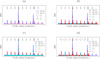 |
Fig. 2 Foundational SES examples are presented with the actual cyclic order αact, the targeted cyclic order αt, and the extraneous cyclic order αext superimposed. (a) compares a baseline SES (SES (B)) against an SES where the CORF is increased (SES (P)). (b) shows the baseline SES with the amplitudes contributing to the signal (SES (B): S) and noise (SES (B): N) indicators. (c) shows the same plot as (b), but the targeted band’s width is decreased. (d) shows the same plot as (b), but an error is introduced in the targeted cyclic order as follows: αt = αc · (1 - error), where the error = 0.2. |
4.2 Selected hyperparameters
In Table 1, the hyperparameters selected for the verification study are presented for the ICS2 and GES2N objectives, summarising the expected impact of hyperparameter changes. The design variables’ starting points and the optimisation approach (i.e., optimisation formulation, optimisation problem and the algorithm) are also hyperparameters in optimal filtering but excluded from the table. The ultimate conclusions should not be affected by the starting points and optimisation approach, and therefore, a two-phased approach is recommended. In the first phase, multiple starting points and different optimisation approaches are tested, whereafter the methods are pruned for a more detailed verification study in the second phase.
In many cases, the sensitivity of the optimal filtering method to the hyperparameters is dataset dependent, e.g., the components in the data, the length of the signal. Figure 2 provides foundational examples to support the explanations in Table 1 and is also used to reinforce the dataset dependency. In Figure 2a, a baseline SES, denoted SES (B), and a SES with a hyperparameter perturbed, denoted SES (P), are shown with the actual cyclic order αact,> the targeted cyclic order αt and the cyclic orders of an extraneous component αext superimposed. The actual cyclic order is the underlying unknown component, whereas αt can be a theoretical or estimated component from the data. Figures 2b-2d also show the amplitudes that contribute to the GES2N’s signal and the noise indicators, denoted SES (B): S and SES (B): N, respectively. An example of the impact of the data can also be inferred; the hyperparameter sensitivity conclusions depend on the targeted and the extraneous components’ characteristics.
The impact of the changes in the hyperparameters on the objective (for a fixed h), the final objective (after the optimal design variable vector h was determined) and the overarching goal (i.e., fault enhancement) could be different. For example, if Δαb is increased, spurious components could contribute to the objective when applying equation (4), which could result in the maximisation of spurious components (which could increase the final objective). Furthermore, increasing the TEP could result in extraneous components to be included in the signal indicator (e.g., Figure 2d), which could be maximised. This could increase the overall objective but impede the enhancement of the fault signature. Table 1 focuses on the final objective unless stated otherwise.
The selected hyperparameter (HP), the expected impact of changing the HP on the ICS2 and the GES2N, and the corresponding motivation are provided.
5 Study outline
The datasets considered in this work are discussed in Section 5.1 and the specific selections for the hyperparameter sensitivity verification analysis are presented in Section 5.2.
5.1 Datasets
The following datasets are used in this study:
Simulated dataset: A simulated dataset enables complete control over the model’s form and components. This control is essential when performing hyperparameter sensitivity verification. The simulated dataset consists of three measurements with different impulse magnification factors (or signal-to-noise ratios). Both ICS2 and GES2N objectives are used on this dataset. Hence, the primary verification is performed using the simulated dataset.
Experimental gearbox dataset: Five measurements, acquired over the life of the damaged gear’s tooth, are considered. These measurements are also used in Ref. [15]. This dataset is more challenging than the simulated dataset and is used to evaluate the parameter sensitivities on experimental data. Only the GES2N objective is used on this dataset for brevity.
5.2 Hyperparameter sensitivity verification analysis
The hyperparameter sensitivity verification analysis is performed in two phases. The first phase is an initial phase, where different optimisation problem formulations and algorithms are used for each objective to confirm their suitability (with the selected settings) and find the optimal filters for each dataset. Thereafter, the hyperparameter sensitivity verification analysis is performed using one suitable optimisation problem formulation and algorithm combination for each parameter perturbation. The initial pruning phase is important to ensure that the optimisation-related hyperparameters are properly selected to obtain reliable results in the verification study. However, the initial pruning phase’s results are not essential for the verification study. Therefore, only the main conclusions from the initial pruning phase are summarised in the main document, while more detailed results are presented in Appendix A.
5.2.1 Optimisation problem formulations and algorithms
Table 2 provides the three optimisation problems, with only one algorithm used for each problem. The labels, which use the algorithm’s name for simplicity’s sake, refer to the combination of the optimisation problem and algorithm used.
The first optimisation problem, labelled CG, consists of an unconstrained problem where the filter coefficients are L2-normalised and are solved using the Conjugate Gradient (CG) algorithm. Problem 2 and 3, respectively labelled SLSQP and IED, are constrained problems solved using the SLSQP and IED algorithms respectively. Problem 3’s objective is written as a non-linear Generalised Rayleigh Quotient (GRQ).
For optimisation problems 1 and 2 in Table 2, the objective function ξ is either the objective ξ(h) = ψ(h) or the natural logarithm of the objective  . The following optimiser settings are used: The maximum number of iterations is 1500, and the convergence tolerance is 10-12 with the settings selected to reduce the impact of the optimiser on the interpretation of the results. Optimisation problem 1 and 2 are solved using analytical gradients. The SES used in subsequent analyses is calculated with equation (2), where the filtered signal
  is calculated with the L2-normalised optimal filter coefficients h/||h||2 . The filter coefficients are normalised to ensure that the SES’ magnitude is invariant to the magnitude of h.
A link to the code repository is supplied in Appendix B, with further information regarding the analytical gradients and the IED optimiser used to solve optimisation problem 3 supplied in Appendix C.
5.2.2 Hyperparameter set
A hyperparameter set is considered for the sensitivity verification for both phases and is presented in Table 3. The following parameters are considered: The filter length D, the number of targeted harmonics Nh, the targeted bandwidth Δαb and the CORF. The CORF is used as follows: Δα = CORF · Δαbase, where Δαbase = π/(θ[L − 1] −θ[0]). The cyclic order TEP relates the actual/correct cyclic order αact with the targeted cyclic order αt as follows:  , with αt used during the optimisation. Lastly, the cyclic order weighting vector of the signal indicator in equation (1) is denoted ws with the four variants and their labels provided in the perturbation column.
The three optimisation problems and selected algorithms are considered in this work. The objective function ξ is either the objective  or the natural logarithm of the objective
  .
.
The hyperparameter (HP) set considered for the sensitivity verification.
5.2.3 Strategy
For the initial pruning phase, the baseline parameters presented in Table 3 are used except for the filter lengths. Three filter lengths  and three different starting points (or initial guesses) are considered for each optimisation problem formulation and algorithm combination. The first starting point, labelled I0 , only consists of one non-zero element at index 0, i.e., h[0] = 1. The second starting point, labelled I1, is equal to the signal’s linear predictive coefficients, and the third starting point, labelled I2, is sampled from an isotropic, zero-mean Ddimensional Gaussian. The objective corresponding to the final design is used to assess and compare the performance of the algorithms, with larger objectives indicating better solutions. The purpose of the comparison is to determine the suitability of the algorithms to find optimal solutions for the different combinations of starting points and filter lengths. The results are pruned, and a suitable combination of problem formulation and algorithm is selected for more in-depth sensitivity verification.
In the second phase, the hyperparameter sensitivity verification study uses the hyperparameter baseline and perturbation set in Table 3. The sensitivity analysis verification is performed by perturbing the hyperparameters OAT around a baseline and quantifying the changes using a metric. OAT results can only be interpreted around the baseline and do not quantify the interdependencies between the parameters or enable selecting the combination of optimal parameters. However, the OAT approach is sufficient to perform the sensitivity verification. To reduce the impact of the optimiser for each specific perturbation, the starting points (I0, I1, I2) that result in the largest final objective are used with the optimisation problem and algorithm selected from the initial phases’ results.
5.2.4 Performance metrics
For the initial phase, the objectives’ logarithm is used as the basis for comparison. For the second phase, two metrics are used. The first metric considered is the logarithm of the ICS2’s objective and is given by:
 (9)
(9)
The second metric is the GES2N metric, which is constructed to be invariant to the magnitude of wi and is defined as follows:
 (10)
(10)
which can be written as  . Since the cyclic band weighting vectors wi are constant during optimisation, the optima of the Mges2n and the GES2N’s objective are the same. In addition to the metrics, the filtered signal’s SES logarithm is visualised for each case, with the SES computed with the cyclic order resolution used during the optimisation. The SES provides further insights into the components enhanced by the filters. The SES for the different perturbations are normalised between 0 and 1 to allow uniformity in colour presentation. For a specific dataset, the metrics are normalised between 0 and 1 using the data from both GES2N and ICS2 objectives, with the normalised metrics denoted
  and
and  respectively. This normalisation makes it easier to compare the methods on the same dataset.
6 Results
The sensitivity verification results of the ICS2 and the GES2N objectives on the simulated dataset are presented in Section 6.1 and the GES2N objectives’ results on the experimental dataset are presented in Section 6.2.
6.1 Simulated dataset
Three simulated signals are generated with
 (11)
(11)
where the train of impulses convolved with the impulse response function h(t) is given by  , with the unit sample function denoted δ(x), i.e., δ(x) = 1 if x = 0 and is 0 otherwise. The time-of-arrival of the kth impulse is denoted Tk and is determined using the instantaneous shaft speed and a characteristic order of 2.0 events/rev. The impulse response function has the form:
  , where the sampling frequency is denoted fs. The ith impulse’s amplitude is given by
  , where ∊G is a standarised Gaussian random variable. The second signal component is given by
  , where φ(t) is the instantaneous phase of the signal. The signal’s amplitude’s dependence on speed is modelled by:
  , where ω(t) is the instantaneous speed of the signal in rad/s and is related to the instantaneous phase as follows
  . Lastly,
  denotes a standardised t-distributed variable with ν degrees-of-freedom. Gaussian-like noise is simulated using the Student-t distribution with νz = 1000 degrees of freedom.
The same speed profile ω(t) = 2π(2.5 · t + 7.5) rad/s was used for all measurements. The three simulated measurements are shown in Figures 3a - 3c respectively. The signals’ duration is 2 seconds and fs = 10000 Hz. Measurements 1-3’s impulse magnification factors κ are 1.5, 3.0, and 10.0 respectively. The ICS2 results are presented in the next section.
6.1.1 ICS2 results
The initial pruning results highlighted that, in general, all methods could result in the same function values if the number of allowable iterations is sufficient. Of the options in Table 2, optimisation problem 3 (the generalised Rayleigh quotient constrained formulation solved using the IED algorithm) was less sensitive to the starting points and therefore used to obtain the sensitivity verification results. The initial pruning results are included in Appendix A.1 for brevity’s sake.
The SES of each filtered signal is shown in Figure 4 with the damage cyclic orders and its harmonics superimposed. The ordinate shows the measurement number and the hyperparameter combination (i.e., whether the baseline or a perturbation is presented). The baseline and perturbations are summarised in Table 3 with all comparisons made relative to the baseline unless stated otherwise.
The damage components’ prominence in the SES and the metric Mics2 increase with measurement number as presented in Figure 4. This makes sense as the impulse magnification factor in the model increased with the measurement number. Furthermore, the damage is not detected for most cases in Measurement 1’s SES, which makes the results (and sensitivity analysis verification) potentially sensitive to spurious noise components, which could impede the conclusions. This result highlights that care should be taken when selecting the measurement for verification.
A summary of the sensitivity verification results of the ICS2 objective is included in Table 4 using  as the basis for comparison. The hyperparameter symbols are defined in Table 1. The check marks indicate that the observed results for the measurements are aligned with the expectations in Table 1. Therefore, the ICS2’s sensitivity is verified on this dataset.
For this dataset, the  metric is generally correlated with the
  metric in Figure 4. There are a few instances where the opposite trends are seen (e.g., for
  ,
,  decreases, whereas
  was unaffected by the perturbations). The metrics are normalised using the ICS2 and GES2N’s data, with the GES2N results presented in the next section, i.e.,
  means it is the largest metric for both objectives. The case with
  is expected since this objective is maximised. Since the GES2N is not maximised,
  for all the cases. This result emphasises that the performance metrics must be carefully selected to ensure a fair comparison is made.
 |
Fig. 3 The three simulated measurements using ω(t) = 2π(2.5 · t + 7.5) rad/s, with the following impulse magnification factors used: 3a: κ = 1.5, 3b: κ = 3.0, and 3c: κ = 10.0. |
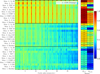 |
Fig. 4 The logarithm of the SES of the filtered signal and the corresponding normalised metrics are presented for three simulated measurements. The filters were obtained by maximising the ICS2 objective. The measurement number and the baseline or perturbation from the baseline are shown on the ordinate. The logarithm of the SES data are normalised between 0 and 1 and the metrics are normalised between 0 and 1 using the ICS2 and GES2N’s data to enable uniformity in colour presentation. |
6.1.2 GES2N results
The initial pruning analysis indicated that optimisation problem 3 performed poorly for the GES2N objective (compared to the other methods). This could be attributed to incomplete tangents being used when applying the IED algorithm as demonstrated in Appendix C. This emphasises that the optimisation approach needs to be well-suited for the problem to ensure a critical comparison can be performed. Optimisation problem 2 (i.e., using the SLSQP algorithm) with the objective’s logarithm is used to find the optimal filters for all hyperparameter perturbations in this section, since it performed well during the initial pruning phase. The initial pruning results for the GES2N are presented in Appendix A.2 for brevity’s sake.
The logarithm of the filtered signals’ SES and corresponding metrics are presented in Figure 5 for the three simulated measurements considered in the previous section. The fault components in the SES and metric  show a general increase with measurement number, consistent with the increased impulse magnification factor. There are larger fluctuations in the SES’ amplitudes for the perturbations compared to the ICS2. This highlights the GES2N is more sensitive to perturbations in the hyperparameters. The fault signatures are generally weak for Measurement 1 with only a few instances seen (e.g., ws : H1 has one prominent harmonic, whereas D = 256 shows multiple harmonics and a larger
  metric). The behaviour of the two metrics is inconsistent in several instances, e.g., for measurement 2, the filter length D perturbations result in different trends. This is because the ICS2 is another proxy for the presence of faults and is not maximised by the GES2N, which re-emphasises the importance of carefully selecting and interpreting metrics for performance evaluation.
The hyperparameter sensitivity verification results are summarised in Table 5 for the considered hyperparameters, with  (not
(not  ) used in the analysis. In some instances, the SES was manually inspected to confirm that the behaviour aligned with the expectation, and only the results are summarised here. The noise indicator is also sensitive to the hyperparameter perturbations, affecting the overall sensitivity in several instances (e.g., if Δαb is too small, the damage component is also partially penalised).
The SES results are consistent with the expectations for the ws perturbations H+, H-, H1, and H1:5 (refer to Table 1 for their definition). The behaviour of the corresponding  is described in more detail here. Generally, the fault harmonics of damaged components show a decreasing trend. If H+ is used, the higher harmonics are enhanced at the expense of the lower harmonics being less enhanced, and the overall metric generally decreases. The H- is more consistent with the typical behaviour of the fault signatures’ SES and therefore
  increases compared to the baseline. H1’s metric generally increases since only one harmonic is used in the objective and the corresponding metric, with the harmonic being prominent despite the higher harmonics being compromised. A similar conclusion is drawn for the H1:5. Hence, the GES2N is verified on the experimental dataset.
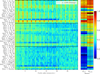 |
Fig. 5 The logarithm of the SES of the filtered signal and the corresponding metrics are presented for three simulated measurements. The filters were obtained by maximising the GES2N objective. |
6.2 Experimental dataset
Five measurements from an experimental gearbox test bench are considered in this section. The experimental test bench, located in the C-AIM laboratory of the University of Pretoria, is shown in Figure 6. The test bench has an electrical motor, alternator, three helical gearboxes, and four shafts (S1 - S4). Gearbox 2 is instrumented with a tri-axial accelerometer, and its input shaft (Shaft S2) is instrumented with a zebra tape shaft encoder and an optical probe for rotational speed measurements. The axial channel of the tri-axial accelerometer is used in this study.
One of gearbox 2’s teeth was seeded with a slot using electrical discharge machining, with the damaged tooth shown in Figure 7a. The experimental tests were performed without disassembling the system between measurements, i.e., the exact gear condition was unknown for the measurements. The gear after the experiment was completed is shown in Figure 7b, with the damaged tooth missing.
The rotational speed of the five measurements is shown in Figure 8 with an example vibration signal. The vibration signal is sampled at 25.6 kHz. Dominant impulsive components in the time domain signal, which manifest at approximately 5.72 shaft orders, impede the fault detection and make it more challenging for damage detection (e.g., refer to [15] for a detailed comparison using these five measurements).
The sensitivity verification in this section only focus on the GES2N’s results. The initial pruning analysis’ results are consistent with the simulated dataset. The optimisation approaches converged to the same final objective except for the optimisation problem 3. This is highlighted not for competition’s sake but to emphasise the importance of ensuring that the selected optimisation approach is appropriate for the objective, hyperparameters and dataset when performing comparisons. The initial pruning results are presented in Appendix A.3 for brevity’s sake.
The parameter sensitivity verification analysis results are presented in Figure 9 for the filtered signals of the five measurements. Similar to the previous section, optimisation problem 2 was used to obtain all the results using the objective’s logarithm and the SLSQP algorithm. The SES’ logarithm and the metrics are shown for the different cases. The ICS2 metric ( ) is low, which is consistent with the simulated dataset. This reinforces the importance of careful performance metric selection. For this dataset, the SES’ logarithm and the GES2N metrics have a bathtub-like behaviour where the damage is less prominent for Measurements 2 and 3, which has also been observed in other analyses (e.g., [45]). However, the hyperparameter sensitivity verification compares the perturbations’ results to the baseline’s for a specific measurement and method.
The sensitivity verification results are presented in Table 6 using the results in Figure 9 and the discussion in Table 1 as a basis. Excluding the ws parameters, all parameter perturbations could be verified. For the H1 perturbations, we found that the first harmonic was made more prominent (which is aligned with our expectations), however, the H1:5, H+ and H- perturbations gave similar results. Since we do not have complete control over the dataset (like the simulated case), and this could be a result of several factors (e.g., the harmonic structure of the fault, the magnitude of the fault components), these perturbations could not be verified. This result emphasises the importance of using simulated datasets when performing hyperparameter sensitivity verification.
 |
Fig. 6 The experimental test bench. (a) The components of the test bench are annotated. (b) The back of the monitored gearbox is visible with the optical probe, zebra tape shaft encoder, and tri-axial accelerometer. |
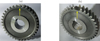 |
Fig. 7 The gear before and after the experiment was completed are shown in Figures 7a and 7b respectively. |
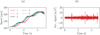 |
Fig. 8 8a shows the rotational speed corresponding to each measurement, 8b shows measurement 5’s vibration signal as an example. |
7 Conclusions
This study establishes the fundamental importance of hyperparameter sensitivity verification in optimal filter design for fault signature enhancement in condition monitoring applications. A key contribution of this work is developing a structured verification framework that can be applied for different optimal filtering problems (e.g., filter coefficient problem, using machine learning) across different datasets and conditions. The framework’s effectiveness is demonstrated by systematically verifying hyperparameter sensitivities in simulated data with controlled fault signatures and applying the framework to real-world gearbox measurements with evolving damage conditions. The analysis verifies the ICS2 and GES2N objectives, with the GES2N showing particular sensitivity to subtle variations in fault signatures under diverse operating conditions. The research also emphasises the hyperparameter sensitivity verification’s dependency on the dataset; it is important to perform the primary evaluation on datasets where all the characteristics can be controlled.
The research provides valuable insights into the behaviour of different hyperparameters, including filter length, cyclic order resolution factors, and targeted bandwidth settings. The study also reveals that the GES2N exhibits greater sensitivity to hyperparameter perturbations than the ICS2, highlighting the critical importance of careful hyperparameter selection and validation when implementing the GES2N. While this increased sensitivity may allow GES2N to be tuned to be a more discriminating tool for fault detection, it also underscores that practitioners must pay particular attention to hyperparameter verification to ensure reliable fault detection can be performed and critical comparisons can be made.
Future work should expand the verification framework to additional simulated and experimental datasets and refine optimisation algorithms to address convergence challenges, particularly for methods like the Iterative Eigenvalue Decomposition approach with the GES2N objective. The findings suggest that the continued development of robust verification methodologies will be crucial for advancing the reliability of condition monitoring and predictive maintenance systems in complex engineering applications.
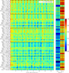 |
Fig. 9 The sensitivity verification results for the GES2N applied on the experimental data. The same format is used as Figure 5 in the simulated dataset. |
Funding
The Article Processing Charges for this article are taken in charge by the French Association of Mechanics (AFM).
Conflicts of interest
The authors have nothing to disclose.
Data availability statement
Data will be made available on request.
Author contribution statement
Conceptualization: S.S., D.N.W., K.G., P.S.H.; Methodology: S.S., D.N.W.; Validation: S.S., D.N.W.; Investigation: S.S., D.N.W.; Software: S.S.; Writing - Original Draft Preparation: S.S., D.N.W.; Writing - Review & Editing, K.G., P.S.H.; Visualization: S.S., D.N.W.
References
- Y. Miao, B. Zhang, J. Lin, M. Zhao, H. Liu, Z. Liu, H. Li, A review on the application of blind deconvolution in machinery fault diagnosis, Mech. Syst. Signal Process. 163, 108202 (2022) [CrossRef] [Google Scholar]
- R.B. Randall, J. Antoni, Rolling element bearing diagnostics - a tutorial, Mech. Syst. Signal Process. 25, 485-520 (2011) [Google Scholar]
- W.A. Smith, P. Borghesani, Q. Ni, K. Wang, Z. Peng, Optimal demodulation-band selection for envelope-based diagnostics: a comparative study of traditional and novel tools, Mech. Syst. Signal Process. 134, 106303 (2019) [CrossRef] [Google Scholar]
- S. Schmidt, K.C. Gryllias, Combining an optimisationbased frequency band identification method with historical data for novelty detection under time-varying operating conditions, Measurement 169, 108517 (2021) [CrossRef] [Google Scholar]
- C. Peeters, J. Antoni, J. Helsen, Blind filters based on envelope spectrum sparsity indicators for bearing and gear vibration-based condition monitoring, Mech. Syst. Signal Process. 138, 106556 (2020) [CrossRef] [Google Scholar]
- W. Su, F. Wang, H. Zhu, Z. Zhang, Z. Guo, Rolling element bearing faults diagnosis based on optimal Morlet wavelet filter and autocorrelation enhancement, Mech. Syst. Signal Process. 24, 1458-1472 (2010) [CrossRef] [Google Scholar]
- R. Wang, X. Ding, D. He, Q. Li, X. Li, J. Tang, W. Huang, Shift-invariant sparse filtering for bearing weak fault signal denoising, IEEE Sensors J. 23, 26096-26106 (2023) [CrossRef] [Google Scholar]
- N.E. Huang, Z. Shen, S.R. Long, M.C. Wu, H.H. Shih, Q. Zheng, N.-C. Yen, C.C. Tung, H.H. Liu, The empirical mode decomposition and the Hilbert spectrum for nonlinear and non-stationary time series analysis, Proc. Math. Phys. Eng. Sci. 454, 903-995 (1998) [CrossRef] [MathSciNet] [Google Scholar]
- D. Abboud, M. Elbadaoui, W. Smith, R. Randall, Advanced bearing diagnostics: A comparative study of two powerful approaches, Mech. Syst. Signal Process. 114, 604-627 (2019) [CrossRef] [Google Scholar]
- D. Abboud, Y. Marnissi, M. Elbadaoui, Optimal filtering of angle-time cyclostationary signals: application to vibrations recorded under nonstationary regimes, Mech. Syst. Signal Process. 145, 106919 (2020) [CrossRef] [Google Scholar]
- L. Wang, W. Ye, Y. Shao, H. Xiao, A new adaptive evolutionary digital filter based on alternately evolutionary rules for fault detection of gear tooth spalling, Mech. Syst. Signal Process. 118, 645-657 (2019) [CrossRef] [Google Scholar]
- X. Jia, M. Zhao, Y. Di, C. Jin, J. Lee, Investigation on the kurtosis filter and the derivation of convolutional sparse filter for impulsive signature enhancement, J. Sound Vibrat. 386, 433-448 (2017) [CrossRef] [Google Scholar]
- P. Borghesani, N. Herwig, J. Antoni, W. Wang, A Fourierbased explanation of 1D-CNNs for machine condition monitoring applications, Mech. Syst. Signal Process. 205, 110865 (2023) [CrossRef] [Google Scholar]
- J. Qin, D. Yang, N. Wang, X. Ni, Convolutional sparse filter with data and mechanism fusion: a few-shot fault diagnosis method for power transformer, Eng. Appl. Artif. Intell. 124, 106606 (2023) [CrossRef] [Google Scholar]
- S. Schmidt, D.N. Wilke, K.C. Gryllias, Generalised envelope spectrum-based signal-to-noise objectives: formulation, optimisation and application for gear fault detection under time-varying speed conditions, Mech. Syst. Signal Process. 224, 111974 (2025) [CrossRef] [Google Scholar]
- M. Buzzoni, J. Antoni, G. d’Elia, Blind deconvolution based on cyclostationarity maximization and its application to fault identification, J. Sound Vibrat. 432, 569-601 (2018) [CrossRef] [Google Scholar]
- K. Kestel, C. Peeters, J. Antoni, J. Helsen, Fault detection via sparsity-based blind filtering on experimental vibration signals, in Annual Conference of the PHM Society, vol. 13 (2021) [CrossRef] [Google Scholar]
- G.L. McDonald, Q. Zhao, Multipoint optimal minimum entropy deconvolution and convolution fix: application to vibration fault detection, Mech. Syst. Signal Process. 82, 461-477 (2017) [CrossRef] [Google Scholar]
- Y. Cheng, B. Chen, G. Mei, Z. Wang, W. Zhang, A novel blind deconvolution method and its application to fault identification, J. Sound Vibrat. 460, 114900 (2019) [CrossRef] [Google Scholar]
- E. Soave, G. D’Elia, M. Cocconcelli, M. Battarra, Blind deconvolution criterion based on Fourier-Bessel series expansion for rolling element bearing diagnostics, Mech. Syst. Signal Process. 169, 108588 (2022) [CrossRef] [Google Scholar]
- B. Zhang, Y. Miao, J. Lin, Y. Yi, Adaptive maximum second-order cyclostationarity blind deconvolution and its application for locomotive bearing fault diagnosis, Mech. Syst. Signal Process. 158, 107736 (2021) [CrossRef] [Google Scholar]
- A. Saltelli, K. Aleksankina, W. Becker, P. Fennell, F. Ferretti, N. Holst, S. Li, Q. Wu, Why so many published sensitivity analyses are false: a systematic review of sensitivity analysis practices, Environ. Model. Softw. 114, 29-39 (2019) [CrossRef] [Google Scholar]
- H. Endo, R. Randall, Enhancement of autoregressive model based gear tooth fault detection technique by the use of minimum entropy deconvolution filter, Mech. Syst. Signal Process. 21, 906-919 (2007) [CrossRef] [Google Scholar]
- C. Lopez, D. Wang, A. Naranjo, K.J. Moore, Box-cox-sparse-measures-based blind filtering: understanding the difference between the maximum kurtosis deconvolution and the minimum entropy deconvolution, Mech. Syst. Signal Process. 165, 108376 (2022) [CrossRef] [Google Scholar]
- Z. Liu, L. Zhang, J. Carrasco, Vibration analysis for largescale wind turbine blade bearing fault detection with an empirical wavelet thresholding method, Renewable Energy 146, 99-110 (2020) [CrossRef] [Google Scholar]
- L. He, D. Wang, C. Yi, Q. Zhou, J. Lin, Extracting cyclostationarity of repetitive transients from envelope spectrum based on prior-unknown blind deconvolution technique, Signal Process. 183, 107997 (2021) [CrossRef] [Google Scholar]
- J. Antoni, The infogram: entropic evidence of the signature of repetitive transients, Mech. Syst. Signal Process. 74, 73-94 (2016) [Google Scholar]
- D. Wang, W.T. Peter, K.L. Tsui, An enhanced kurtogram method for fault diagnosis of rolling element bearings, Mech. Syst. Signal Process. 35, 176-199 (2013) [CrossRef] [Google Scholar]
- J. Lin, L. Qu, Feature extraction based on Morlet wavelet and its application for mechanical fault diagnosis, J. Sound Vibrat. 234, 135-148 (2000) [CrossRef] [Google Scholar]
- K. Kestel, C. Peeters, J. Antoni, Q. Leclere, F. Girardin, J. Helsen, Informed sparsity-based blind filtering in the presence of second-order cyclostationary noise, Mech. Syst. Signal Process. 199, 110438 (2023) [CrossRef] [Google Scholar]
- L. He, C. Yi, D. Wang, F. Wang, J.-H. Lin, Optimized minimum generalized Lp/Lq deconvolution for recovering repetitive impacts from a vibration mixture, Measurement 168, 108329 (2021) [CrossRef] [Google Scholar]
- P. Borghesani, J. Antoni, CS2 analysis in presence of nongaussian background noise-effect on traditional estimators and resilience of log-envelope indicators, Mech. Syst. Signal Process. 90, 378-398 (2017) [CrossRef] [Google Scholar]
- P. Borghesani, P. Pennacchi, S. Chatterton, R. Ricci, The velocity synchronous discrete Fourier transform for order tracking in the field of rotating machinery, Mech. Syst. Signal Process. 44, 118-133 (2014) [CrossRef] [Google Scholar]
- S. Chauhan, G. Vashishtha, R. Zimroz, R. Kumar, M.K. Gupta, Optimal filter design using mountain gazelle optimizer driven by novel sparsity index and its application to fault diagnosis, Appl. Acoust. 225, 110200 (2024) [CrossRef] [Google Scholar]
- D. Economou, C. Mavroidis, I. Antoniadis, C. Lee, Maximally robust input preconditioning for residual vibration suppression using low-pass fir digital filters, J. Dyn. Syst. Meas. Control 124, 85-97 (2002) [CrossRef] [Google Scholar]
- T. Parks, J. McClellan, Chebyshev approximation for nonrecursive digital filters with linear phase, IEEE Trans. Circuit Theory 19, 189-194 (1972) [CrossRef] [Google Scholar]
- Z. Zhou, B. Chen, B. Huang, W. Zhang, F. Gu, A.D. Ball, X. Gong, Maximum negative entropy deconvolution and its application to bearing condition monitoring, Struct. Health Monitor. 14759217231181679 (2023) [Google Scholar]
- S. Schmidt, P.S. Heyns, K.C. Gryllias, An informative frequency band identification framework for gearbox fault diagnosis under time-varying operating conditions, Mech. Syst. Signal Process. 158, 107771 (2021) [CrossRef] [Google Scholar]
- W.N. Niehaus, S. Schmidt, P.S. Heyns, NIC methodology: a probabilistic methodology for improved informative frequency band identification by utilizing the available healthy historical data under time-varying operating conditions, J. Sound Vibrat. 488, 115642 (2020) [CrossRef] [Google Scholar]
- A. Mauricio, W.A. Smith, R.B. Randall, J. Antoni, K. Gryllias, Improved envelope spectrum via feature optimisation-gram (IESFOgram): a novel tool for rolling element bearing diagnostics under non-stationary operating conditions, Mech. Syst. Signal Process. 144, 106891 (2020) [CrossRef] [Google Scholar]
- J.A. Snyman, D.N. Wilke, Practical mathematical optimization: basic optimization theory and gradient-based algorithms, Springer Optimization and Its Applications (SOIA), vol. 133 (2018) [CrossRef] [Google Scholar]
- D.N. Wilke, S. Kok, J.A. Snyman, A.A. Groenwold, Gradient-only approaches to avoid spurious local minima in unconstrained optimization, Optim. Eng. 14, 275-304 (2013) [CrossRef] [MathSciNet] [Google Scholar]
- E. Borgonovo, E. Plischke, Sensitivity analysis: a review of recent advances, Eur. J. Oper. Res. 248, 869-887 (2016) [CrossRef] [Google Scholar]
- P. Virtanen, R. Gommers, T.E. Oliphant, M. Haberland, T. Reddy, D. Cournapeau, E. Burovski, P. Peterson, W. Weckesser, J. Bright, S.J. van der Walt, M. Brett, J. Wilson, K.J. Millman, N. Mayorov, A.R.J. Nelson, E. Jones, R. Kern, E. Larson, C.J. Carey, I. Polat, Y. Feng, E.W. Moore, J. VanderPlas, D. Laxalde, J. Perktold, R. Cimrman, I. Henriksen, E.A. Quintero, C.R. Harris, A.M. Archibald, A.H. Ribeiro, F. Pedregosa, P. van Mulbregt, SciPy 1.0 Contributors, SciPy 1.0: fundamental Algorithms for Scientific Computing in Python, Nat. Methods 17, 261-272 (2020) [NASA ADS] [CrossRef] [Google Scholar]
- S. Schmidt, R. Zimroz, P.S. Heyns, Enhancing gearbox vibration signals under time-varying operating conditions by combining a whitening procedure and a synchronous processing method, Mech. Syst. Signal Process. 156, 107668 (2021) [CrossRef] [Google Scholar]
Cite this article as: S. Schmidt, D. N. Wilke, P. S. Heyns, K. C. Gryllias Verifying hyperparameter sensitivities of optimal filter design methods for fault signature enhancement, Mechanics & Industry 26, 22 (2025), https://doi.org/10.1051/meca/2025014
Appendix A Initial pruning results
The initial pruning results are presented here for the different datasets and objectives. The ICS2 and GES2N results on the simulated datasets are presented in Sections A.1 and A.2, whereas the GES2N’s results on the experimental datasets are presented in Section A.3.
A.1 Dataset 1 - ICS2’s results
The initial phase’s results using the ICS2 objective are presented in Figure A.1 for three stages of the optimisation process, namely, after completing 10 iterations, 50 iterations, and the final results (i.e., after the optimiser terminated). The normalised log10 of the objective is presented with the colour bar, with the values normalised to make the comparisons easier. The measurement number and algorithms, coupled with the optimisation problem formulation in Table 2, are listed on the ordinate. The abscissa shows the filter length and the filter starting points combinations.
The final function evaluation results show that most combinations of optimisation problem formulations and algorithms converged to the same solution when using the same filter length and filter starting point. Shorter filter lengths (e.g., D = 16) have lower function values than the longer filter lengths (e.g., D = 64), with the difference between D = 64 and D = 256 being more subtle. This objective’s increase with filter length aligns with our expectations. Similar results were obtained after 50 function evaluations. Some cases have not converged after 10 function evaluations, emphasising that sufficient iterations are needed to ensure that the conclusions are independent of the optimiser. The results highlight that more prominent damage might result in faster convergence than weaker damage. The IED (i.e., using the generalised Rayleigh quotient constrained formulation and IED algorithm) is the only optimisation problem formulation and algorithm combination that converged for all starting points and will, therefore, be used for the parameter sensitivity verification.
A.2 Dataset 1 - GES2N’s results
The initial phase’s results for the GES2N objective are presented in Figure A.2. Excluding the IED’s results (i.e., optimisation formulation 3), the final objectives are independent of the starting points, with the objective increasing with filter length and measurement number. The objective is expected to increase with filter length and measurement number because a longer filter has more flexibility to enhance the signal-to-noise ratio, and the impulse magnification factor (and signal-to-noise ratio) increases with measurement number.
After 50 function evaluations, the optimiser only converged for shorter filter lengths (i.e., D = 16), with significant variation still seen for longer filter lengths. Similar trends are observed after 10 function evaluations. The results make sense since longer filters have more unknowns and is expected to require more iterations and function evaluations to converge.
In contrast to the ICS2, the IED algorithm could not converge for the GES2N objective when using longer filter lengths, despite the ICS2 and the GES2N having the same numerators. Finding a better solver for the GES2N’s optimisation problem 3 is left for future work. The constrained problem formulation using the logarithm of the objective and the SLSQP solver performed well and is used in the parameter verification study.
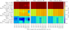 |
Fig. A.1 The normalised logarithm of the final ICS2 objective for the three simulated measurements is shown for different hyperparameters. Different combinations of optimisation problem formulations and algorithms are shown on the ordinate, and the filter length D and filter starting points I0, I1 and I2 are shown on the abscissa. Three stages are presented: The objective after 10 function evaluations (left), the objective after 50 function evaluations (middle) and the final objective’s value (right). For example, if the optimiser terminated before 50 function evaluations, the converged solution is presented in the middle plot. |
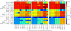 |
Fig. A.2 The normalised logarithm of the final GES2N objective for the three simulated measurements is shown for different hyperparameters. |
A.3 Dataset 2 - GES2N’s results
The initial phase’s results of optimising the GES2N on the experimental data are presented in Figure A.3. The same procedure was followed as Section A.2. The final results (the right plot) are consistent with the simulated data; except for the IED algorithm, all optimisers could converge to the same function values. This highlights that the optimisation settings are sufficient to reduce the impact of the optimiser. This is corroborated by the significant variation in the objectives after 10 and 50 function evaluations, which show some optimisers have not converged. The same solver was used as for Dataset 1’s GES2N objective.
Appendix B Code repository
The following code repository is made available to enhance the reproducibility of the results: https://gitlab.com/vspa/hparmsv4of.
Appendix C Additional optimisation information
C.1 Analytical gradients
Analytical gradients are used to solve optimisation problems 1 and 2. The analytical gradient of an objective with the form  is given by
 (C.1)
(C.1)
whereas the gradient of the objectives’ logarithm is given by
 (C.2)
(C.2)
C.2 Optimisation problem 3’s solution
Optimisation problem 3 considers objectives written as nonlinear generalised Rayleigh quotients
 (C.3)
(C.3)
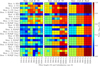 |
Fig. A.3 The normalised logarithm of the final GES2N objective for the five experimental measurements (Case 1) is shown for different optimisation problem formulation and algorithm combinations, filter lengths and starting points. |
where  . The Lagrangian is defined as follows for the equivalent minimisation problem:
 (C.4)
(C.4)
where λ denotes the Lagrangian multiplier. The optimality criteria of the optimisation problem can be used to find the solution of λ and h [41]:
 (C.5)
(C.5)
 (C.6)
(C.6)
This reduces equation (C.5) to the following equation if A(h) and B(h) are symmetric:
 (C.7)
(C.7)
with  . Equation (C.7) can be written as follows:
 (C.8)
(C.8)
with  and
and  . Hence, it is a non-linear eigenvalue problem with an eigenvalue λ and the corresponding eigenvector h.
If  , equation (C.8) can be further simplified as the following generalised eigenvalue problem:
 (C.9)
(C.9)
where  is the eigenvalue of the simplified problem. By premultiplying equation (C.9) with hT, we can show
  , and therefore the eigenvector that corresponds to the largest eigenvalue is used as the solution.
The Iterative generalised Eigenvalue Decomposition (IED) algorithm solves equation (C.9) as follows:
For k = 0, supply a starting point h0, and proceed with the next step by setting k = 1.
-
For iteration k, find hk by solving the following generalised eigenvalue problem:

where hk-1 is the solution at the previous iteration k - 1, i.e., the matrices A(hk-1) and B(hk-1) are not updated when solving the eigenvalue problem.
Increase k by 1 and repeat step 2 until the termination criteria are satisfied.
This is an equivalent algorithm used in Refs. [5,16,24] according to our knowledge. Note, when this IED algorithm is used, some terms in equation (C.7) are missing, i.e., the tangents are incomplete. This can potentially affect the convergence of the method, with a more in-depth analysis left for future work.
All Tables
The selected hyperparameter (HP), the expected impact of changing the HP on the ICS2 and the GES2N, and the corresponding motivation are provided.
The three optimisation problems and selected algorithms are considered in this work. The objective function ξ is either the objective or the natural logarithm of the objective .
All Figures
|
Fig. 1 This conceptual framework illustrates an optimal filtering workflow, starting with raw input signals and progressing through pre-processing, transformations, objective definition, and optimisation towards performance evaluation. On the left, various methods of preparing and transforming signals are shown, while the centre section focuses on formulating the optimisation problem and selecting suitable optimisation algorithms. Performance metrics and approaches for evaluating filter quality are presented on the right. Below, a HyperParameter (HP) sensitivity verification strategy ensures robust and verified filter designs. Abbreviations: AR: Auto-Regressive, CG: Congjugate Gradient, HT: Hilbert Transform, ICS2: Indicator of second-order CycloStationarity, QN: Quasi-Newton, RMSE: Root-Mean-Squared Error, SES: Squared Envelope Spectrum, SN: Spectral Negentropy, SNR: Signal-toNoise Ratio, SQP: Sequential Quadratic Programming, STFT: Short-Time Fourier Transform, WT: Wavelet Transform. |
| In the text | |
|
Fig. 2 Foundational SES examples are presented with the actual cyclic order αact, the targeted cyclic order αt, and the extraneous cyclic order αext superimposed. (a) compares a baseline SES (SES (B)) against an SES where the CORF is increased (SES (P)). (b) shows the baseline SES with the amplitudes contributing to the signal (SES (B): S) and noise (SES (B): N) indicators. (c) shows the same plot as (b), but the targeted band’s width is decreased. (d) shows the same plot as (b), but an error is introduced in the targeted cyclic order as follows: αt = αc · (1 - error), where the error = 0.2. |
| In the text | |
|
Fig. 3 The three simulated measurements using ω(t) = 2π(2.5 · t + 7.5) rad/s, with the following impulse magnification factors used: 3a: κ = 1.5, 3b: κ = 3.0, and 3c: κ = 10.0. |
| In the text | |
|
Fig. 4 The logarithm of the SES of the filtered signal and the corresponding normalised metrics are presented for three simulated measurements. The filters were obtained by maximising the ICS2 objective. The measurement number and the baseline or perturbation from the baseline are shown on the ordinate. The logarithm of the SES data are normalised between 0 and 1 and the metrics are normalised between 0 and 1 using the ICS2 and GES2N’s data to enable uniformity in colour presentation. |
| In the text | |
|
Fig. 5 The logarithm of the SES of the filtered signal and the corresponding metrics are presented for three simulated measurements. The filters were obtained by maximising the GES2N objective. |
| In the text | |
|
Fig. 6 The experimental test bench. (a) The components of the test bench are annotated. (b) The back of the monitored gearbox is visible with the optical probe, zebra tape shaft encoder, and tri-axial accelerometer. |
| In the text | |
|
Fig. 7 The gear before and after the experiment was completed are shown in Figures 7a and 7b respectively. |
| In the text | |
|
Fig. 8 8a shows the rotational speed corresponding to each measurement, 8b shows measurement 5’s vibration signal as an example. |
| In the text | |
|
Fig. 9 The sensitivity verification results for the GES2N applied on the experimental data. The same format is used as Figure 5 in the simulated dataset. |
| In the text | |
|
Fig. A.1 The normalised logarithm of the final ICS2 objective for the three simulated measurements is shown for different hyperparameters. Different combinations of optimisation problem formulations and algorithms are shown on the ordinate, and the filter length D and filter starting points I0, I1 and I2 are shown on the abscissa. Three stages are presented: The objective after 10 function evaluations (left), the objective after 50 function evaluations (middle) and the final objective’s value (right). For example, if the optimiser terminated before 50 function evaluations, the converged solution is presented in the middle plot. |
| In the text | |
|
Fig. A.2 The normalised logarithm of the final GES2N objective for the three simulated measurements is shown for different hyperparameters. |
| In the text | |
|
Fig. A.3 The normalised logarithm of the final GES2N objective for the five experimental measurements (Case 1) is shown for different optimisation problem formulation and algorithm combinations, filter lengths and starting points. |
| In the text | |
Current usage metrics show cumulative count of Article Views (full-text article views including HTML views, PDF and ePub downloads, according to the available data) and Abstracts Views on Vision4Press platform.
Data correspond to usage on the plateform after 2015. The current usage metrics is available 48-96 hours after online publication and is updated daily on week days.
Initial download of the metrics may take a while.