


| Issue |
Mechanics & Industry
Volume 27, 2026
Overview of recent advances in research for next generation in Mechanical Engineering
|
|
|---|---|---|
| Article Number | 32 | |
| Number of page(s) | 14 | |
| DOI | https://doi.org/10.1051/meca/2026029 | |
| Published online | 01 July 2026 | |
Original Article
Simplified modeling of a wooden vehicle restraint system to reduce computation time
Univ Gustave Eiffel, Univ Lyon 1, LBMC UMR_T 9406, Lyon, France
* e-mail: This email address is being protected from spambots. You need JavaScript enabled to view it.
Received:
29
October
2025
Accepted:
29
May
2026
Abstract
Vehicle restraint systems (VRS) are components installed on roadsides or freeways to ensure the safety of road users. The validation of a VRS is conditioned by crash tests in accordance with standards EN 1317-1 and EN 1317-2. Due to the high cost of crash testing, manufacturers rely on their experience, analytical calculations, and upstream numerical simulations to design VRS that meet the standards before experimental validation. However, these simulations can have a high computational cost. Therefore, the aim of this study is to propose a simplified model of a wooden VRS, close to a reference numerical model, enabling a significant reduction in computational time. The proposed design comprises rails and posts connected by joints, with a solid wood rail made up of 2-m-long elements. Numerical simulations show that this design satisfies the TB32 test, corresponding to a 1500 kg vehicle launched at 110 km/h with an impact angle of 20°. However, as the computational time is strongly influenced by the assemblies, a reference model with a continuous rail has been proposed, constituting a first simplification. The results indicate that only the parts of the VRS close to the impact zone are subject to high levels of deformation. Consequently, it is possible to simplify the parts remote from this zone in order to further optimize the computational time. Three approaches are proposed to represent these parts: the LS model replaces the remote zones with longitudinal springs; the LTS model uses longitudinal and transverse springs; and the beam (B) model uses the remote parts using beam-type finite elements. All three simplified models are validated and are able to reproduce the reference model with a continuous rail. The EN 1317-1 and EN 1317-2 criteria and the computational time show that the B model is closer to the reference model than the other two. In particular, the computational time is reduced by a factor of approximately 1.8 for the simplified models, while maintaining good agreement with the reference results. The B model, therefore, provides a good representation of the reference model at a lower computational cost.
Key words: Vehicle restraint systems / computational time / numerical simulation / crash test / simplified modeling / wood / LS-DYNA
© C.J. Nyobe et al., Published by EDP Sciences, 2026
 This is an Open Access article distributed under the terms of the Creative Commons Attribution License (https://creativecommons.org/licenses/by/4.0), which permits unrestricted use, distribution, and reproduction in any medium, provided the original work is properly cited.
1 Introduction
A vehicle restraint system (VRS) is a piece of road safety equipment designed to limit vehicle run-off, reduce the severity of accidents, and thus protect road users. They must comply with European standards for the construction and design of road safety barriers [1,2]. The validation of VRSs is subject to crash tests in accordance with EN 1317-2 [2], which defines performance classes, crash test acceptance criteria, and test methods for VRSs. Given the high financial and material costs associated with crash testing, manufacturers prefer to use their expertise, analytical calculations, and numerical simulations in the design phase in order to design devices that comply with the standards before their experimental validation. This approach considerably reduces the number of actual tests required while optimizing the development process. Numerical simulations make it possible to analyze the behavior of VRSs under a variety of conditions, test different configurations, and identify critical areas for improvement [3].
In recent years, significant progress has been made in the numerical simulation of VRSs. Several studies have demonstrated that finite element models can accurately reproduce full-scale crash tests and provide reliable predictions of barrier performance. For example, Palta et al. [4] showed that high-fidelity numerical models can reproduce experimental crash responses with good agreement in terms of vehicle trajectories, structural deformations, and safety indicators. Similarly, Fang et al. [5] highlighted the capability of detailed numerical models to evaluate the performance of multi-rail barrier systems under MASH standards and to identify potential design limitations under different impact conditions. In addition, advanced numerical approaches now incorporate detailed modeling of occupant safety, including indicators such as HIC (head injury criteria), OIV (occupant impact velocity), and THIV (theoretical head impact velocity), allowing a more comprehensive evaluation of crashworthiness [6]. Recent studies have also emphasized the importance of considering realistic configurations, such as sloped terrains, which can significantly affect barrier performance [7].
However, these high-fidelity numerical models are generally associated with a very high computational cost. They often involve several hundreds of thousands to millions of finite elements, complex contact definitions, and nonlinear material behaviors. As a result, these approaches require significant computational resources and lead to long computational times, which limits their applicability for parametric studies, optimization processes, or sensitivity analyses.
Few studies have been carried out on wooden VRSs. The first VRS, called “Tulip”, with restraint level H2 (vehicle speed: 70 km/h, impact angle: 20°, and vehicle mass: 13000 kg), was developed in the Netherlands [8,9]. The second was designed by Pilia [10]. This VRS successfully passed the TB11 numerical simulation test (vehicle mass: 900 kg, speed: 100 km/h, and impact angle: 20°).
Tabiei and Wu [11] have highlighted three major challenges in VRS modeling: bolted connections, which significantly influence the transmission of forces between barrier elements; post–soil interaction, which plays an important role in VRS response; and the effect of VRS ends, which simplifies the simulation of parts of the barrier far from the impact zone. In this work, we focus on the simulation of wooden VRSs and more specifically on the latest challenge.
The length of the barrier must be sufficient to cover the portion of the road undergoing the crash test. A tested VRS can be up to a hundred meters long, and the use of finite elements can generate considerable computational costs. To overcome this limitation, Tabiei and Wu [11] proposed a simplification approach consisting of modeling only the part of the VRS directly subjected to impact. In this approach, areas of the VRS remote from the impact zone are not modeled explicitly but replaced by longitudinal elastic springs, simulating the continuity of the structure in both directions. The cross-section of the unmodeled part of the W-beam is assumed to remain in the elastic domain during impact. The stiffness of the longitudinal springs is determined by the mechanical properties of the material and the geometry of the barrier. Spring stiffness is determined by the mechanical properties of the material and the barrier geometry. More precisely, it is proportional to the modulus of elasticity of the material and the cross-sectional area of the beam and inversely proportional to the length of the nonmodeled part of the VRS. This method is widely used in the literature to model parts of the VRS remote from the impact zone [12–15]. In fact, these laws do not take into account several important factors, such as posts, connections between the rails and posts, and post–soil interaction. This makes it impossible to accurately reproduce the behavior of the VRS.
Nevertheless, these simplified approaches may neglect important physical phenomena, such as structural connections, post behavior, and soil–structure interaction, which can significantly influence the global response of the system. Furthermore, most of these approaches have been developed for steel barriers and are not directly adapted to wooden VRSs, which exhibit specific mechanical behaviors.
Simplifying the VRS model will decrease the computational time of a crash test. This is useful for designing a wooden VRS. Indeed, as many parameters are uncertain, a sensitivity analysis is necessary to assess the robustness of the design. However, a sensitivity study of a VRS would require approximately 100 simulations and then would generate considerable computational time. One solution could be to incorporate simplification methods adapted to wood VRSs, such as those used for steel VRSs.
This limitation becomes critical when using high-fidelity numerical models, where each simulation is computationally expensive. Therefore, there is a clear need for simplified modeling approaches that can significantly reduce computational cost while maintaining sufficient accuracy. The novelty of this work lies in the development of simplified modeling strategies specifically adapted to wooden VRSs, accounting for connections, posts, and soil interaction while significantly reducing computational cost.
The aim of this article is to propose a simplified model of a wooden VRS, enabling computational time to be reduced while remaining faithful to a reference model. To achieve this objective, we first present in Section 2 the design of the VRS, where the wooden rails and posts are connected by bolted joints. Next, in Section 3, a model with a continuous rail is proposed to eliminate the connections, thus constituting an initial simplification: this model will be considered as the reference model. Three simplified models are then developed to reduce the length of the VRS by simplifying the modeling of parts far from the impact zone. They are presented in Section 4.
Finally, a comparative study between the reference model and the simplified models will be carried out in Section 5.
The models considered in this study are publicly available on Zenodo [16]. Therefore, the following section focuses on their main principles and essential features, whereas comprehensive descriptions and full technical details can be found in the corresponding repository.
2 VRS design and modeling
2.1 VRS design
The design of the VRS involves determining the dimensions, shapes, and arrangements of its components, such as rails, posts, and assemblies.
2.1.1 Rails and posts
The posts are 1829 mm long, of which 1016 mm are embedded in the ground. Their rectangular cross-section is 200 × 100 mm. They are spaced at intervals of 2 m. The rails have a rectangular cross-section of 250 × 200 mm and a length of 2 m. The distance between the ground and the bottom of the rails is 450 mm.
2.1.2 Assemblies
Bolts and metal plates are used to join the rails to the posts (Fig. 1). The metal plates are 10 and 6 mm thick, respectively. Ten class 8.8 M16 bolts are used for the connections, spaced at intervals of 100 mm in the longitudinal direction and 90 mm in the vertical direction.
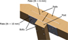 |
Fig. 1 Post-rail assembly. |
2.1.3 Barrier length
The studied barrier has a total length of 65 m and is composed of 30 posts and 30 beam elements. This length is selected in accordance with EN 1317-2 recommendations, which require that the barrier be long enough to avoid any lateral deflection of the ends of the installed barrier [2].
The discontinuous rail model (DR model) of this design, which will be subjected to the TB32 test, will be presented in Section 2.2.
2.2 Discontinuous rail model
Figure 2a illustrates the modeling of the device used for the TB32 crash test (vehicle speed: 111.4 km/h, vehicle mass: 1454 kg, and impact angle: 20°). Further details are provided in Figure 2b. The modeling of the various elements is carried out using LS-DYNA software and will be detailed in the following paragraphs.
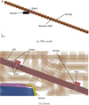 |
Fig. 2 TB32 test modeling. |
2.2.1 Rails and posts
Rails and posts are represented by a finite element model using 8-node solid hexahedral elements, with a mesh size of 25 mm. Goubel [17] showed that the mesh refinement of wood materials had a limited influence on the simulation results. A mesh sensitivity study was not conducted, as previous work demonstrated the limited influence of mesh refinement for wood materials in similar configurations. The posts are discretized using 2340 elements for each post, while the complete rail is modeled with 84,480 elements.
The constitutive law *MAT_WOOD_PINE, available in LS-DYNA, has been assigned to the posts and rails, as it is an orthotropic material model specifically developed for wood, accounting for its anisotropic and nonlinear behavior under dynamic loading, which makes it suitable for crash simulations [18]. The model also incorporates strain-rate effects and failure mechanisms, making it suitable for impact simulations of wooden structures. The input parameters are listed in Table 1.
Wood input parameters and associated hourglass parameters.
2.2.2 Bolts and metal plates
The metal plates are modeled by shells, meshed with 4-node elements, with a mesh size of 30 mm. The plates are made of S235 steel, modeled with LS-DYNA’s *MAT_PIECEWISE_LINEAR_PLASTICITY behavior law. The input parameters for the metal plates are summarized in Table 2.
Bolts with a circular cross-section are modeled using Hughes–Liu beam elements [17,19,20]. This formulation allows an efficient representation of their mechanical behavior while reducing computational cost. The most suitable material model in LS-DYNA for these elements is *MAT_PLASTIC_KINEMATIC [21]. They are meshed with 25 mm elements. The bolt input parameters are listed in Table 3.
The connection between bolts and wooden elements is provided by the coupling *BEAM_IN_SOLID, which allows an efficient transfer of forces between beam and solid elements while maintaining numerical stability. The connection between bolts and metal plates is modeled using the keyword *CONTACT_SPOTWELD, available in LS-DYNA, as it is well suited to represent localized connections between components.
Rail–plate, plate–post, and vehicle–VRS contacts are defined using the *AUTOMATIC_SURFACE_TO_SURFACE, with a type 2 SOFT constraint, which is widely used in crash simulations due to its robustness and its ability to handle complex interactions between multiple deformable bodies under large deformations [22].
Static and dynamic friction coefficients are set at 0.2. The friction coefficient (0.2) is consistent with values commonly reported in the literature for vehicle–barrier interactions and ensures stable and realistic contact behavior [17,23,24].
Input parameters for metal plates (*MAT_PIECEWISE_LINEAR_PLASTICITY card).
Bolt input parameters (*MAT_PLASTIC_KINEMATIC card).
2.2.3 Vehicle and contacts
The vehicle used was developed by the Laboratoire INRETS Équipement de la Route (LIER, now Transpolis) to represent a TB32 test vehicle. In the context of numerical simulations, the vehicle model is defined in accordance with EN 16303 [25], which specifies the requirements for virtual testing. The considered vehicle has a mass of 1454 kg and a velocity of 111.4 km/h. These values comply with the standard requirements for a TB32 test, which specifies a vehicle mass of 1500 ± 75 kg and an impact velocity of 110 km/h with a lower tolerance of 0% and upper tolerance of 7%. The model is composed of 21,306 finite elements.
2.2.4 Post–soil interaction
In this work, the soil is modeled by springs (Fig. 2b) [13,15,24]. The springs are attached to the post in the horizontal (longitudinal and lateral) and vertical directions. In the horizontal direction, the springs are attached to all nodes on two adjacent sides of the post, located below the ground surface. In the vertical direction, the springs are attached to the underside of the post. The first spring node, N1, is attached to the post, while the second node, N2, is placed in the ground (i.e. N2 = 0 in LS-DYNA). More details can be found in [23,26].
To determine the constitutive law of nonlinear springs, a numerical compression test was carried out. The test consists in compressing the soil contained in a reservoir using a rigid solid, applied at a constant speed of 1.67 × 10⁻¹ ms−1. The resultant of the forces exerted by the soil on the solid was recorded, as well as the displacement of the rigid solid. The force–displacement curve obtained (Fig. 3) is then used as the constitutive law of springs.
Figure 3 represents the law F(d), describing the evolution of the resultant force exerted by the soil on the rigid body as a function of displacement during the compression test. This force results from the contact pressure exerted by the soil on the rigid body over the contact surface, whose area is denoted by A.
The objective is to determine the constitutive law of N identical springs representing the pressure exerted by the soil on the post through their contact surface, whose area is denoted by B. The constitutive law of a single spring attached to the post, FN(d), is therefore derived from the law F(d) as follows:
 (1)
(1)
A summary of the material models used for the different components of the VRS and the vehicle is provided in Table 4.
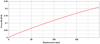 |
Fig. 3 Constitutive law of springs. |
Summary of material models used in the simulations.
2.3 DR model verification
Verification [27] can be defined as the set of activities defined to check whether a numerical model is numerically reliable and stable [25]. It consists firstly in verifying the code (establishing the assurance, through the collection of evidence, that the mathematical model and solution algorithms work correctly) and secondly in verifying the calculations (establishing the assurance, through the collection of evidence, that the discrete solution of the mathematical model is accurate in relation to the standard). According to EN 16303 [25], a numerical simulation is verified if the following criteria are justified:
The total energy of the analysis solution (i.e., kinetic, potential, contact, etc.) must not vary by more than 10% from the beginning, also taking into account the eroded energy;
The zero deformation energy (hourglass) of the analysis solution is, at all times, less than 5% of the total initial energy at the start of the stroke;
The zero deformation energy (hourglass) of the analysis solution at the end of the stroke is less than 10% of the total internal energy at the end of the stroke;
The mass added to the model in its entirety is less than 5% of the mass of the model in its entirety at the start of the run;
All contact energies must be positive.
Figure 4 summarizes these energies. Based on these energies, the following observations have been drawn:
Variation in total energy between the beginning (764 kJ) and end (760 kJ) of the analysis is less than 10%;
The energy of the hourglass (21.1 kJ) at the end of the analysis is less than 5% of the total energy (760 kJ) at the end of the analysis;
The energy of the hourglass (21.1 kJ) at the end of the stroke is less than 10% of the total internal energy (223 kJ) at the end of the stroke;
The contact energy is positive.
In conclusion, as these criteria have been met, the simulation is verified.
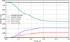 |
Fig. 4 DR model energies. |
2.4 DR-VRS TB32 crash-test validation
Crash-test validation criteria are essential to ensure that VRSs provide effective protection for occupants and reduce the risk of serious injury in the event of an accident. This validation is based on a comparison of crash test results with the performance requirements defined in EN 1317-1. These requirements include an acceleration severity index (ASI) less than or equal to 1.90, a THIV less than or equal to 33 km/h, and a vehicle exit angle not exceeding 25.2°.
Two parameters, dynamic deflection and working width, are taken into account when assessing the performance of a VRS. Dynamic deflection (Dm) corresponds to the maximum deformation of the front face of the VRS exposed to traffic. The working width (Wm) is the lateral distance within which the VRS can deform or move under the impact of a vehicle without posing a danger to other road users or adjacent structures.
Table 5 summarizes these criteria from the numerical simulation of a TB32 test on the DR wooden barrier modeled in Section 2.2. As all criteria are met, the DR-VRS numerical model passes the TB32 test.
DR-VRS and CR-VRS TB32 crash-test validation.
3 Continuous rail model
Computational time is strongly influenced by the connection modeling. A model with a continuous rail (CR model) is proposed to reduce computational time. This simplification is justified by the fact that the connections between rail segments are designed to be sufficiently rigid to ensure effective force and moment transfer. Therefore, the barrier can be reasonably modeled as a continuous structure without significantly altering its global behavior.
This model allows us to replace all the 2 m rails with a continuous rail, which reduces computational time by simplifying the modeling of the connections between the rails on the one hand and between the rails and the posts on the other hand.
3.1 CR model presentation
The CR model is identical to the one presented in Section 2.2, with the exception of the metal plates, which are removed, and the rail, which is considered continuous. Post–soil interaction is defined as in Section 2.2.4, and vehicle-VRS contact is defined using the *AUTOMATIC_SURFACE_TO_SURFACE card, with a type 2 SOFT stress. Static and dynamic friction coefficients are set at 0.2.
3.2 CR model verification
Figure 5 shows the energies of the CR model. Based on these energies, the following observations have been drawn:
Variation in total energy between the beginning (764 kJ) and the end (762 kJ) of the analysis is less than 10%;
The energy of the hourglass (21.3 kJ) at the end of the analysis is less than 5% of the total energy (762 kJ) at the end of the analysis;
The energy of the hourglass (21.3 kJ) at the end of the stroke is less than 10% of the total internal energy (218 kJ) at the end of the stroke;
The contact energy is positive.
In conclusion, since these criteria have been met, the CR model simulation has been verified.
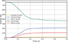 |
Fig. 5 CR model energies. |
3.3 CR-VRS TB32 crash-test validation
The objective is to validate the CR model with respect to the DR model in the context of the TB32 crash-test. Table 5 summarizes the criteria in accordance with EN 1317-1 [1] and EN 1317-2 [2] that must be compared.
Standard EN 16303 [25] defines the validation criteria for ensuring that the results obtained by simulation (virtual testing) are reliable and consistent with the real tests. In our case, the DR model of Section 2.2 is considered to be the real test; the CR model is considered to be the virtual test. We denote by DDR the dynamic deflection measured during the real test and by DCR that obtained from the virtual test. Table 6 shows the results of the comparison between the DR model and the CR model.
With all these criteria verified, we can conclude that the CR model faithfully represents the DR model. In addition, it significantly reduces the computational cost, with simulation time decreasing from 1 h 41 min 48 s for the DR model to 1 h 21 min 27 s for the CR model. This CR model therefore constitutes a first level of simplification of the DR model, enabling a substantial reduction in simulation time while preserving the essential physical behavior. It will also serve as the basis for a second simplification step, which will focus on the extremities of the VRS, with the objective of further optimizing the model while maintaining sufficient accuracy.
Simulations were performed on a high-performance computing cluster using compute nodes with 48 CPU cores (two 24-core AMD EPYC 7F72 processors) and 256 GB of memory. Parallel computations were carried out using the MPP (massively parallel processing) version of LS-DYNA (version 4.13) on a distributed-memory architecture, enabling efficient scaling over multiple cores.
CR model validation.
4 Simplified models
In crash tests, only the parts of the VRS located in the impact zone undergo significant deformation. Areas far from the impact zone, on the other hand, are only slightly affected. This means that the length of the VRS can be reduced by simplifying the modeling of the less stressed parts. Figure 6 shows the areas of the VRS that will be simplified (before and after the impact zone). The length of the reduced VRS was defined so as to isolate the impact influence zone [11]. The upstream and downstream truncation limits are determined as the first locations, measured from the impact zone, at which the horizontal deformation of the VRS, evaluated after the impact, falls below 3% of the maximum dynamic deflection and remains below this threshold over the remaining length.
Three simplified models are proposed: the longitudinal spring (LS) model, in which zones far from the impact zone are replaced by longitudinal springs; the longitudinal plus transverse spring (LTS) model, where they are replaced by longitudinal and transverse springs; and the beam (B) model, where they are replaced by beam-type finite elements.
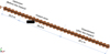 |
Fig. 6 Parts far from the impact zone. |
4.1 Model with longitudinal springs and model with longitudinal plus transverse springs
The VRSs are identical to the reference model presented in Section 3, with the exception of the zones away from the impact zone, which are replaced by longitudinal springs (LS model; Fig. 7a), or by longitudinal and transverse springs (LTS model; Fig. 7b). The first nodes of the springs are merged with the nodes of the 3D rail, and the second nodes are fixed.
The constitutive laws of the transverse and longitudinal springs (Fig. 7d) are obtained from quasi-static tests performed on the substituted zones of the VRS. The test consists of subjecting one end of these zones to a constant speed of 1.67 × 10⁻³ ms−1, while the other end remains fixed. The speed was chosen because, in quasi-static testing, the strain rate must remain below 0.1 s−1. Force and displacement at the points where speed is imposed are recorded, in both longitudinal and transverse directions. L-Upstream and L-Downstream (Fig. 8a) correspond, respectively, to the force–displacement curves in the longitudinal direction before and after the impact zone of the VRS, while T-Upstream and T-Downstream (Fig. 8b) represent those in the transverse direction, also before and after the impact zone. Note that L-Upstream and L-Downstream have different stiffnesses due to the variation in length of the zones concerned (see Fig. 6).
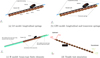 |
Fig. 7 Simplified models. |
 |
Fig. 8 Spring constitutive laws. |
4.2 Beam model
In the B model, the VRS elements (rail and post) located in the impact zone are modeled by 3D solids, as described in Section 3, whereas rails and posts are replaced by finite beam elements, i.e., 1D elements (Fig. 7c), in the other zones. The nodes located at the junction between the rails and the posts are merged. The rectangular cross-section characteristics of the rails (200 × 250 mm) and posts (200 × 100 mm) are mentioned in the *SECTION_BEAM card, and the behavior law *MAT_PIECEWISE_LINEAR_PLASTICITY is assigned to them. The input parameters for beam-type finite elements, which are those for wood, are given in Table 7.
The connection between the 3D solid elements and the finite beam elements is provided by a metal plate in the plane of the beam section. The nodes of the plate are merged with those of the nodes of the 3D beam cross-section and welded to the beam finite elements by LS-DYNA’s *CONTACT_SPOTWELD card. The metal plate is a shell of thickness 5 mm and is associated with the behavior law *MAT_RIGID (density: 7850 kg/m3, Young’s modulus: 210,000 MPa, and Poisson’s ratio: 0.3).
Input parameters for beam-type finite elements (*MAT_PIECEWISE_LINEAR_PLASTICITY card).
4.3 Verification of the LS, LTS, and B models
Figure 9 shows the energies of the simplified models. Table 8 summarizes the verification criteria for simplified model simulations. As all the criteria are met, the simulations are verified.
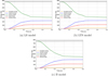 |
Fig. 9 Energies of the LS, LTS, and B models. |
Verification of simplified models.
4.4 TB32 crash test validation of simplified models
The aim is to validate the tests simulated using the simplified models against those carried out using the CR model in accordance with standard EN 16303: the continuous rail model is considered to represent the real test, while the simplified models are considered to be the simulated models. Table 9 summarizes the values of the criteria to be validated. Table 10 presents the results of the comparison between the reference model and the simplified models. It can be seen that all the criteria pass the validation test; therefore, it can be concluded that the simplified models can be substituted for the reference model. It can also be noted that the VRS modeled using the simplified models passes the TB32 test.
Performance criteria for models CR, LS, LTS, and B.
Validation of TB32 simulations of the simplified LS, LTS, and B models against the CR model (Si stands for simplified).
5 Comparative study of different models
5.1 Comparison criteria
The three simplified LS, LTS, and B models are compared with the reference model, which is the CR model, according to several criteria: computational time, TB32 test performance criteria, and maximum displacements of the rail points close to the top of four posts.
5.2 Simulation time
Table 11 summarizes the modeling and computational time data for the different models. It can be seen that the CR model has about twice as many elements as the simplified models.
This reduction in the number of elements reduces the number of degrees of freedom to be calculated and, consequently, the computational time. This is confirmed by the fact that the computational time of the simplified models is reduced by a factor of approximately 1.8 compared with the reference model.
Simulation data for models CR, LS, LTS, and B.
5.3 TB32 test performance criteria
The results of the simplified LS, LTS, and B models (Tab. 9) show excellent correspondence with the CR model on all validation criteria. ASI remains constant at 0.8 for all models. The THIV values are also close to those of the reference model (27.6 km/h): the LS and LTS models have 27.9 km/h, while the B model is slightly lower at 27.7 km/h; they are all well below the 33 km/h limit. As for dynamic deflection, the simplified models range from 409 mm (B model) to 415 mm (LS model), while the CR model has a deflection of 407 mm, with minor differences. The working width varies between 704 and 711 mm for the simplified models, against 702 mm for the CR model: the differences are small and remain below 1.2%. Finally, the output box is identical for all models at 4.2°, well below the 25.2° limit.
5.4 The maximum displacements of the rail points at the four posts
The simplified models were also evaluated by comparing the displacements of points located on the rail at the level of four posts with those of the reference model (Fig. 10a). To this end, displacement curves were obtained for posts 0, 1, 2, and 3. Figures 10b–10d illustrate the time evolution of these displacements along the three axes of the VRS: longitudinal (l), transverse (t), and vertical (z).
The displacement curves along the longitudinal axis show that model B is the closest to the reference model, with root mean square error (RMSE) values ranging from 0.1 to 0.3 mm (see Tab. 12), compared with a maximum displacement of 4.3 mm for the CR model. The RMSE values of the LS and LTS models range from 0.7 to 1.1 mm and 0.7 to 1.1mm, respectively (Tab. 12). Figure 10d confirms that the displacement curves obtained with the B model are in good agreement with those of the reference model. Since the longitudinal displacement is small compared with the transverse displacement, these deviations have a limited impact on the overall horizontal displacement, which is dominated by the transverse component.
The comparison in the transverse direction reveals significant differences in absolute deviations between the simplified models and the CR model. However, these deviations should be considered in relation to the maximum transverse displacement of 365.6 mm observed for the CR model. The B model exhibits moderate deviations, with values ranging from 4.9 to 6.7 mm. These relatively small deviations demonstrate the ability of the B model to accurately reproduce the transverse displacements obtained with the CR model. The corresponding curves remain close to the reference curves. The LS model shows larger deviations, with values reaching 25.6 mm. The largest deviations are observed for the LTS model, with values reaching 31.5 mm at post 2 and 22.7 mm at post 1.
The maximum vertical displacement observed for the CR model is 25.2 mm. Once again, the B model provides the closest agreement with the reference model in the vertical direction, with values ranging from 0.3 to 0.6 mm. The LTS model shows larger errors, with values reaching 3.8 mm at post 2, although its curves remain globally close to the reference. The LS model exhibits global consistency with values reaching 3.7 mm at post 2, indicating noticeable differences in vertical displacements. This trend is also clearly visible in the displacement curves, where the discrepancy between the LS and LTS models and the reference model is more pronounced than for the B model.
Overall, the B model appears to be the most accurate, providing the best agreement with the reference model in all three directions while more faithfully reproducing the global structural behavior.
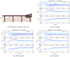 |
Fig. 10 Displacements at the top of the posts (solid line: LS, LTS, and B models; dashed line: reference model with continuous rail). |
Comparison of RMSE (millimeter) to evaluate the simplified models (full scale for bar values is 31.52, which is the maximum value).
5.5 Conclusions on the various simplified models
Replacing the portions of the VRS far from the impact zone with three simplified models led to a reduction in computational time by a factor of approximately 1.8, with a similar gain observed for all three approaches.
In addition, all simplified models show good agreement with the reference model in terms of TB32 test criteria. However, the B model exhibits the smallest deviations in terms of dynamic deflection, working width, and THIV, making it the closest simplified representation with respect to these global indicators.
A more detailed analysis of the displacement responses highlights a more nuanced behavior. Since the transverse displacement governs the overall structural response, it constitutes the most relevant indicator for model assessment. In this direction, all simplified models exhibit limited deviations from the reference model, and their responses remain globally consistent. In contrast, larger relative errors are observed in the longitudinal and vertical directions. The B model consistently shows the best agreement with the reference model across the different displacement components, while the LS and LTS models present larger discrepancies depending on the considered direction.
A sensitivity study typically requires a large number of simulations. In this context, the cross-sections of springs and posts may vary between configurations, requiring the identification of constitutive laws for the LS and LTS models in each case, which makes their implementation relatively cumbersome. In contrast, the B model allows direct modification of the cross-section through the *SECTION_SOLID card, significantly simplifying its use.
Overall, the B model appears to provide the best compromise between accuracy and computational efficiency, particularly when considering global performance indicators, while the LS and LTS models offer slightly improved consistency in certain displacement components.
These results highlight the relevance of simplified modeling strategies for reducing computational cost while preserving the global behavior of the VRS. In particular, the good performance of the B model can be attributed to its ability to retain structural continuity while reducing the number of degrees of freedom. From an industrial perspective, this approach is especially well suited for parametric studies and design optimization, where a large number of simulations are required. However, the proposed simplifications rely on assumptions regarding the behavior of the VRS portions located far from the impact zone, which may limit their applicability to other configurations or loading conditions.
This behavior can be further interpreted in light of the physical mechanisms involved during impact. During the impact event, loads are progressively redistributed along the VRS through the rail and the posts, involving both axial force transfer and bending effects. These mechanisms are only partially captured by simplified spring-based representations. As a result, such models tend to localize the response near the impact zone, whereas beam-based formulations allow a more realistic propagation of forces and deformations along the structure.
This also contributes to explaining the differences observed in energy dissipation (Fig. 9), as the simplified models do not fully capture the combined effects of structural continuity and soil–structure interaction on the overall energy absorption mechanisms.
6 Conclusion
A wooden VRS, made up of rails and posts connected by bolted joints and capable of passing the TB32 test, was presented. This work enabled us to present and evaluate several simplified models of the VRS, with the aim of reducing computational time while maintaining good accuracy compared with the initial model.
The introduction of a model with a continuous rail was a valid first simplification, allowing us to optimize the modeling by eliminating the connections between rails without altering the representativeness of the VRS’s behavior.
The study then focused on three models designed to simplify modeling of the portions of the VRS remote from the impact zone: the LS model, incorporating longitudinal springs; the LTS model, adding transverse springs; and the B model, where these parts are replaced by beam-type finite elements. The results show that the B model is the most faithful to the reference model, with minimal differences in terms of dynamic deflection and working width. In addition, it achieves a reduction in computational time of approximately 1.8 times with respect to the model with continuous rails; this reduction is more or less the same for the other two models.
Finally, if a sensitivity analysis requiring hundreds of simulations must be carried out, it is much quicker to modify the characteristics of the B model than those of the LS and LTS models. Indeed, the LS and LTS models require determination of the spring behavior laws for each simulation, making the approach more tedious. The B model, on the other hand, considerably simplifies this task by allowing direct modification of the cross-section in LS-DYNA *SECTION_SOLID card.
As a result, the B model appears to be the most accurate and efficient, ensuring an optimal compromise between accuracy and computational time. Following on from this work, a sensitivity study will be carried out to analyze the influence of the VRS parameters on the results. This analysis will enable us to better understand the factors influencing the robustness of the model to further refine its performance.
Future work will focus on extending the proposed approach to a wider range of impact conditions, barrier geometries, and vehicle types in order to assess its general applicability.
Acknowledgments
The authors would like to thank Transpolis for accepting to share online the vehicle model used for this study.
Funding
The authors declare that they have not received any funding for this study.
Conflicts of interest
The authors declare that they have no conflict of interest.
Data availability statement
The data that support the findings of this study are available from the corresponding author, upon reasonable request.
Additionaly, the LS-DYNA models of this study are openly available in Zenodo [16].
Author contribution statement
Charly Julien Nyobe: Writing—original draft, Investigation, and Software; Eric Jacquelin: Writing—review & editing and Supervision; Denis Brizard: Writing—review & editing, Software, and Supervision; Alexy Mercier: Writing—review & editing and Supervision.
References
- Road restraint systems - Part 1 : terminology and general criteria for test methods, EN 1317-1 (2010) [Google Scholar]
- Road restraint systems - Part 2: Performance classes, impact test acceptance criteria and test methods for safety barriers including vehicle parapets, EN 1317-2 (2010) [Google Scholar]
- T.Y. Yosef, R.K. Faller, C. Fang, S. Kim, A state-of-the-art review on computational modeling of dynamic soil–structure interaction in crash test simulations, Geotechnics 4, 127–157 (2024) [Google Scholar]
- E. Palta, H. Fang, C. Stolle, Q. Wang, Experimental and numerical crashworthiness evaluation of a two-bar bridge rail, Eng. Struct. 340, 120753 (2025) [Google Scholar]
- H. Fang, C. Jaus, Q. Wang, E. Palta, L. Pachocki, D. Bruski, Numerical modeling and simulation of vehicular crashes into three-bar metal bridge rail, Computation 12, 165 (2024) [Google Scholar]
- E. Palta, L. Pachocki, D. Bruski, Q. Wang, C. Jaus, H. Fang, Finite element analysis of occupant risk in vehicular impacts into cluster mailboxes, Computation 13, 12 (2025) [Google Scholar]
- Q. Wang, E. Palta, H. Fang, Numerical modeling and simulation of cable barriers under vehicular impacts on a sloped median, Int. J. Prot. Struct. 15, 891–916 (2024) [Google Scholar]
- J. van de Kuilen, The first full timber guardrail for highways Erste Leitplanke aus Vollholz für Straßenklasse Autobahn, Technical Report (2012) [Google Scholar]
- J.W.G. van de Kuilen, V. Antonelli, I.C. de Pauw, A timber guardrail for highways made with hardwoods, in: Proceedings of the 7th International Scientific Conference on Hardwood Processing, Delft University of Technology, The Netherlands 278–285 (2019) [Google Scholar]
- F. Pilia, F. Maltinti, F. Annunziata, Preliminary results on a new safety road barrier made completely of wood. Environ. Semeiot. 5, 11–23 (2012) [Google Scholar]
- A. Tabiei, J. Wu, Roadmap for crashworthiness finite element simulation of roadside safety structures, Finite Elem. Anal. Des. 34, 145–157 (2000) [Google Scholar]
- Z. Ren, M. Vesenjak, Computational and experimental crash analysis of the road safety barrier, Eng. Fail. Anal. 12, 963–973 (2005) [Google Scholar]
- M. Borovinšek, M. Vesenjak, M. Ulbin, Z. Ren, Simulation of crash tests for high containment levels of road safety barriers, Eng. Fail. Anal. 14, 1711–1718 (2007) [Google Scholar]
- T.-L. Teng, C.-C. Liang, T.-T. Tran, Development and validation of a finite element model for road safety barrier impact tests, Simulation 92, 565–578 (2016) [Google Scholar]
- T.-L. Teng, Impact performance of W-beam guardrail supported by different shaped posts, Int. J. Mech. Eng. Appl. 4, 59 (2016) [Google Scholar]
- C.J. Nyobe, E. Jacquelin, A. Mercier, D. Brizard. Simplified vehicle restraint systems LS-DYNA models (2026). Available from: https://doi.org/10.5281/zenodo.19854032 [Google Scholar]
- C. Goubel, Vehicle restraint system crash test modelling: Application to steel-wood structures, PhD Thesis, Université de Lyon, France, 2012 [Google Scholar]
- Y.D. Murray, Manual for LS-DYNA wood material model 143 (2007) [Google Scholar]
- M. Hadjioannou, D. Stevens, M. Barsotti, Development and validation of bolted connection modeling in LS-DYNA for large vehicle models, in LS-DYNA for large vehicle models, in: Proceedings of the 14th International LS-DYNA User Conference, Dearborn, USA, 1–12 (2016) [Google Scholar]
- M. Mongiardini, WP5 – Computational Mechanics Modelling of Bolt Connections for the ESP-N2 Barrier. Main Report, Vol. 1 of 1, Technical Report, Doc. No. ROBUST-05-016c, Rev. 0 (2005) [Google Scholar]
- LS-DYNA® Keyword User’s Manual, Vol. II: Material Models, Technical Report (2017) [Google Scholar]
- S. Bala, J. Day, General guidelines for crash analysis in LS-DYNA, Livermore Software Technology Corporation (2012) [Google Scholar]
- C. Nyobe, Contribution à l’élaboration de dispositifs de retenue de route entièrement ou partiellement en bois, PhD Thesis, Université Gustave Eiffel, France, (2025) [Google Scholar]
- B. Bhattacharyya, Uncertainty quantification and propagation in rapid dynamics : application to crash problem, PhD Thesis, Université de Lyon, France, (2020) [Google Scholar]
- Road restraint systems - Verification and validation process for the use of virtual tests in vehicle restraint impact tests, EN 16303, (2020) [Google Scholar]
- C.J. Nyobe, E. Jacquelin, D. Brizard, A. Mercier, Simplified modeling of post-soil interaction for roadside safety barriers, in: Proceedings of the International Conference on Traffic and Transportation Engineering, New York, NY, USA, 2025 [Google Scholar]
- L.E. Schwer, An overview of the PTC 60/V&V 10: guide for verification and validation in computational solid mechanics: Transmitted by L. E. Schwer, Chair PTC 60/V&V 10, Eng. Comput. 23, 245–252 (2007) [Google Scholar]
Cite this article as: C.J. Nyobe, E. Jacquelin, A Mercier, D. Brizard, Simplified modeling of a wooden vehicle restraint system to reduce computation time, Mechanics & Industry 27, 32 (2026), https://doi.org/10.1051/meca/2026029
All Tables
Input parameters for beam-type finite elements (*MAT_PIECEWISE_LINEAR_PLASTICITY card).
Validation of TB32 simulations of the simplified LS, LTS, and B models against the CR model (Si stands for simplified).
Comparison of RMSE (millimeter) to evaluate the simplified models (full scale for bar values is 31.52, which is the maximum value).
All Figures
|
Fig. 1 Post-rail assembly. |
| In the text | |
|
Fig. 2 TB32 test modeling. |
| In the text | |
|
Fig. 3 Constitutive law of springs. |
| In the text | |
|
Fig. 4 DR model energies. |
| In the text | |
|
Fig. 5 CR model energies. |
| In the text | |
|
Fig. 6 Parts far from the impact zone. |
| In the text | |
|
Fig. 7 Simplified models. |
| In the text | |
|
Fig. 8 Spring constitutive laws. |
| In the text | |
|
Fig. 9 Energies of the LS, LTS, and B models. |
| In the text | |
|
Fig. 10 Displacements at the top of the posts (solid line: LS, LTS, and B models; dashed line: reference model with continuous rail). |
| In the text | |
Current usage metrics show cumulative count of Article Views (full-text article views including HTML views, PDF and ePub downloads, according to the available data) and Abstracts Views on Vision4Press platform.
Data correspond to usage on the plateform after 2015. The current usage metrics is available 48-96 hours after online publication and is updated daily on week days.
Initial download of the metrics may take a while.