© J. Lepagneul et al., Published by EDP Sciences 2026

1 Introduction

Transition from fossil energies to all‐electric machines in industry spurs the substitution of most conventional engines by electric ones. As a consequence of this technological shift, hydraulic networks are opportunely superseded by electric ones with benefits in maintainability, volume and reliability. In this context, linear hydraulic actuators are progressively substituted by electro‐mechanical actuators (EMA).

Except linear motors, most electro‐mechanical actuators are made of an engine fitted with mechanical converters to modify its rapid rotational motion to the target motion, often translation. Planetary roller‐screw mechanisms (PRSMs) are rotation‐translation motion converters. They have a similar role as conventional ballscrews but with enhanced performances in terms of load capacity, fatigue lifespan, reduction of mass and volume [1].

An exploded view of an inverted PRSM is shown in Figure 1. Standard or inverted PRSMs are compounded of the same elements: a nut (1‐green), several rollers (4‐light grey), and a screw (3‐blue). The rollers are set in place by two carriers (2‐red) to avoid roller‐roller collision. Finally, the carriers are translation‐locked with two circlip rings (5‐grey). Standard and inverted PRSM have different kinematics. Rollers engage around the nut (no net translation between nut and rollers) for standard PRSM whereas rollers engage around the screw for an inverted one (no net translation between screw and rollers). The kinematics of standard and inverted PRSMs are shown in Figure 2.

Because PRSMs are considered key in aerospace and defense, they are under intense research efforts to understand their functioning [2–4] mainly displacement accuracy, dynamical behaviour, friction torque and mechanical damage. Recent works focused on mechanism compliance and load distribution among thread contacts with joint analytical/numerical approaches [5–10], machine learning approach [11] or finite element modelling [6, 11,12]. Most research works pointed out that the load distribution among threads is not uniform and depends on the loading configuration. Besides mechanism compliance, the second source of thread load variability originates from machining errors [7,11,13]. However, experiments are difficult to perform on PRSM and little experimental data is reported in the literature except some notable exceptions [9,10,14,15].

Electromechanical, mechanical or hydraulic actuators were used to create loading experimentally. Abevi et al. [15] measured the position of each roller and screw regarding nut using high precision capacitive sensors. The mechanism stiffness was changed by varying the number of rollers. The two other experimental benches focused directly on the global PRSM stiffness (displacement between screw and nut). Guo et al. [9] used an inductive sensor and Ma et al. [10] used a linear grating ruler. These two last experimental benches present an offset between the measure and loading axes. Furthermore, capacitive or inductive sensors require clean environments without dust or electromagnetic perturbations. In this paper, the global PRSM stiffness (between screw and nut) was characterized changing the number of rollers and the number of contact points per roller.

The variability of loads at thread contacts plays a role on the lifetime of a PRSM. Meng et al. [16] studied the wear at the thread contact for accuracy displacement considering local loads and Archard's law. The PRSM thread wear has also been investigated under extreme functioning [17] showing degradation at the thread contacts in lubricated and unlubricated conditions. The wear at thread contact was measured experimentally by Zhang et al. [13] and corresponded to thread contact overload due to machining errors. More refined contact modelling including rolling and sliding phenomenon were computed. Du et al. [7] estimated the fatigue lifetime of a compliant PRSM under classical loads considering pressure criterion.

Thread contacts have been shown to present normal and tangential loads. Normal loads create maximal shear in bulk and sliding changes the depth of the maximal shear. In rare extreme sliding conditions, it can move up to the surface. To consider this complex loading, a multiaxial criterion must be considered to define the fatigue lifespan [18].

In our previous work, the fatigue lifetime of a PRSM was invistigated under uniform loading at thread contacts [19]. In this paper, this assumption is relaxed and the fatigue lifespan of a PRSM is considered including mechanism compliance and a microscopic multi‐axial criterion for crack initiation [18]. To validate the compliant model, an experimental test bench was proposed to quantify global PRSM stiffness. It has been developed to comply with basic precision engineering principle (Abbe's principle) and using a new generation displacement sensor of high accuracy (confocal measurement principle). Similarly to Abevi et al. [15], the number of rollers was changed, but we also tested a new configuration were the number of contacts per roller is modified.

The paper is organised as follows: First, a direct modelling of PRSM displacements is proposed. This predictive modelling, without fitting parameter, is a full analytical pipeline from mechanism design to load distribution among thread contacts. Second this modelling is proof‐checked with independent experimental tests about the global stiffness of the PRSM. Finally, we use our modelling to predict the fatigue lifetime of a PRSM using Dang‐Van criterion for fatigue.

Fig. 1 Components of an inverted PRSM. The nut (1‐green) encloses rollers (4‐light grey) and screw (3‐blue). The rollers are placed in contact with the screw by two carriers (2‐red) which are in pivot joint with the screw and locked by two circlip rings (5‐grey).

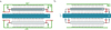Fig. 2 Diagram of PRSM kinematics. a. Standard PRMS. Rollers do not translate regarding nut. b. Inverted PRSM. Rollers do not translate regarding screw. N‐green : Nut. R‐grey : Rollers. S‐blue: Screw. C‐red: Carriers. Punctual contacts are shown with arrows and circles.

2 Multiscale modelling of load distribution in PRSMs

The load distribution is not uniform among thread contacts and varies with the locus of the external load [5,7,12]. The first step to predict the lifetime of a PRSM is to determine the location of the maximal contact load. Four loading modes are possible for a PRSM as shown in Figure 3a. The external load (black arrow) may be positive, negative or alternate. To take into account the mechanism compliance, we modified the modelling of Jones and Velinsky [5] to directly describe mechanism displacements rather than deformations. The model appears lighter without reference to classical finite element framework. The model considers bulk stiffness of the roller k_R, the screw k_S and the nut k_N and contact stiffness between roller‐nut k_NR and roller‐screw threads k_SR. The schematic of the model is shown in Figure 3b.

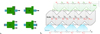Fig. 3 a. Experimental loading configurations. Green: nut. Blue: screw. A (Top‐left): External load on screw and clamped nut on same side. B (Top‐right): External load on screw and clamped nut on opposite side. C (Bottom‐left): External load on nut and clamped screw on opposite side. D (Bottom‐right): External load on nut and clamped screw on same side. b. Modelling of a compliant PRSM (configuration A) inspired from [5]. Only one equivalent roller is shown. The nut (resp. screw) has n contacts with the equivalent roller. 5 different springs are considered: bulk nut kN, bulk screw kS, bulk roller kR, roller‐screw contact kSR and roller‐nut contact kNR.

2.1 Bulk and contact stiffness

A single equivalent roller is shown considering all rollers being in parallel. Bulk stiffness are found considering one‐dimensional Hooke law between two consecutive contact positions,

$$k_N=\frac{\pi E\left(r_{\text{ext}}^2-r_N^2\right)}{p},k_S=\frac{\pi E{r}_S^2}{p}and{k}_R=\frac{2\pi n_{R}E{r}_R^2}{p}$$(1)

with p the mechanism pitch, E mechanism Young's modulus, r_N (resp. r_S, r_R) the nut (resp. screw, roller) nominal radius and n_R the number of rollers (see Tab. 1 for a complete list of parameters). Factor 2 in bulk roller stiffness is a consequence of consecutive contacts on the roller being only separated by half a pitch (nut contact on one side and screw contact on the other).

Contact between solids is often modelled as non‐linear with a 3/2 power law (Hertz contact), f = αx^3/2 where f is the contact load and x is the indentation. α is a constant which depends on contact geometry and mechanical properties of the solids. The α computation algorithm is given in 7. Non‐linear Hertz contacts are difficult to treat with efficient tools of linear algebra. In order to simplify the problem, Hertz contact is linearized around the uniform force distribution at the contact, $\widehat{f}=F/n{n}_R$. The linearized contact force reads (see Appendix B for details),

$$f=kx-\frac{\widehat{f}}{2}\text{with}k=\frac{3{ɑ}^{2/3}{\widehat{f}}^{1/3}}{2}\mathrm{.}$$(2)

Thus equivalent contact stiffness is the sum of individual stiffness over the number of rollers,

$$k_{SR}=\frac{3n_R}{2}{ɑ}_{SR}^{2/3}{\widehat{f}}^{1/3}\text{and}{k}_{NR}=\frac{3n_R}{2}{ɑ}_{SR}^{2/3}{\widehat{f}}^{1/3}\mathrm{.}$$(3)

The typical values of bulk stiffness and contact stiffness used in the model are given in Table 3. Note that contact stiffness k_NR and k_SR given in Table 3 are for information only. For each load level F, the linearized Hertz contact are computed around $\widehat{f}=F/n{n}_R$ from equation (3).

2.2 Static equilibrium

Except on the edges, $\forall i\in [2;n-1]$ the static equilibrium of each section of nut, screw and equivalent roller reads,

$$\begin{array}{ll}\text{Nut}:\hfill & k_N(N_{i+1}-N_{i-1}-2N_i)+k_{NR}(R_{2i-1}-N_i)-\widehat{f}{n}_R/2=0\hfill \\ \text{Roller}:\hfill & \{\begin{array}{l}{k}_R(R_{2i+1}+R_{2i-1}-2R_{2i})+k_{SR}(S_i-R_{2i})-\widehat{f}{n}_R/2=0\hfill \\ k_R(R_{2i+2}+R_{2i}-2R_{2i+1})-k_{NR}(R_{2i+1}-N_{i+1})+\widehat{f}{n}_R/2=0\hfill \end{array}\hfill \\ \text{Screw}:\hfill & k_S(S_{i+1}+S_{i-1}-2S_i)-k_{SR}(S_i-R_{2i})+\widehat{f}{n}_R/2=0\hfill \end{array}$$(4)

where N_i, S_i and R_i are nut, screw and equivalent roller positions along the axis, see Figure 3b. Two distinct equations are set for the roller describing the fact that each side is either in contact with the nut or the screw.

The equivalent roller static equilibria at edges read simply,

$$\begin{array}{ll}\text{for}i=1:\hfill & -k_{NR}(R_1-N_1)+\widehat{f}{n}_R/2+k_R(R_2-R_1-p/2)=0\hfill \\ \text{for}i=2n:\hfill & k_{SR}(S_n-R_{2n})-\widehat{f}{n}_R/2-k_R(R_{2n}-R_{2n-1}-p/2)=0.\hfill \end{array}$$(5)

The screw and nut boundaries depend on loading configuration. For the loading configuration of interest here, with external load applied on the screw and clamped nut on the same side, see Figure 3a top‐left, boundary conditions read

$$\begin{array}{l}{k}_N(N_2-N_1-p)+k_{NR}(R_1-N_1)-\widehat{f}{n}_R/2=0\hfill \\ N_n=0\hfill \\ k_S(S_2-S_1-p)+k_{SR}(S_1-R_2)+\widehat{f}{n}_R/2=0\hfill \\ F-k_S(S_n-S_{n-1}-p)-k_{SR}(S_n-R_{2n})+\widehat{f}{n}_R/2=0\hfill \end{array}.$$(6)

The boundary conditions, corresponding to other loading configurations of the PRSM are given in Appendix B.

We now leverage on linear algebra tools to solve this system of linear equations. The system of equations (4), (5) and (6) simply read

$$KX-(P+F)=0\text{with}X=\left(\begin{array}{c}\hfill N_1\hfill \\ \hfill N_2\hfill \\ \hfill ⋮\hfill \\ \hfill N_{n-1}\hfill \\ \hfill N_n\hfill \\ \hfill R_1\hfill \\ \hfill R_2\hfill \\ \hfill ⋮\hfill \\ \hfill R_{2n-1}\hfill \\ \hfill R_{2n}\hfill \\ \hfill S_1\hfill \\ \hfill S_2\hfill \\ \hfill ⋮\hfill \\ \hfill S_{n-1}\hfill \\ \hfill S_n\hfill \end{array}\right),F=\frac{\widehat{f}{n}_R}{2}\left(\begin{array}{c}\hfill 1\hfill \\ \hfill 1\hfill \\ \hfill ⋮\hfill \\ \hfill 1\hfill \\ \hfill 0\hfill \\ \hfill {(-1)}^1\hfill \\ \hfill {(-1)}^2\hfill \\ \hfill ⋮\hfill \\ \hfill {(-1)}^{2n-1}\hfill \\ \hfill {(-1)}^{2n}\hfill \\ \hfill -1\hfill \\ \hfill -1\hfill \\ \hfill ⋮\hfill \\ \hfill -1\hfill \\ \hfill -1-2F/\widehat{f}\hfill \end{array}\right),\text{and}P=p\left(\begin{array}{c}\hfill k_N\hfill \\ \hfill 0\hfill \\ \hfill ⋮\hfill \\ \hfill 0\hfill \\ \hfill 0\hfill \\ \hfill k_R/2\hfill \\ \hfill 0\hfill \\ \hfill ⋮\hfill \\ \hfill 0\hfill \\ \hfill -k_R/2\hfill \\ \hfill k_S\hfill \\ \hfill 0\hfill \\ \hfill ⋮\hfill \\ \hfill 0\hfill \\ \hfill -k_S\hfill \end{array}\right)\mathrm{.}$$(7)

This system is solved for positions by inverting the stiffness matrix K,

$$X=K^{-1}\left(P+F\right).$$(8)

Once deformed positions are found, the local forces on threads read,

$$f_{SR,i}=\frac{k_{SR}}{n_R}\left(S_i-R_{2i}\right)-\frac{\widehat{f}}{2},\text{and}{f}_{NR,i}=\frac{k_{NR}}{n_R}\left(R_{2i-1}-N_i\right)-\frac{\widehat{f}}{2}.$$(9)

3 Experimental validation of PRSM global stiffness

PRSM is a complex macro‐mechanism with numerous contact points. It is difficult to monitor contact forces between threads directly. However, we can consider convenient displacements to compare theoretical and experimental results.

3.1 Experimental set‐up

The dimensions and geometric parameters of the PRSM of interest are given in Table 2. Contact points and contact geometry (curvatures and main directions) were computed from the design parameters using the algorithm described in Lepagneul et al. [19]. Contact geometries comprising 4 main curvatures and angles between eigen‐frames are given in Table 2. These values are used to compute contact stiffness from the algorithm given in Appendix A. The bulk and contact stiffness are given in Table 4 for $\widehat{f}$ = 75 N (F = 15 kN for 8 rollers and 25 contacts per rollers).

The traction test bench is shown in Figure 4. The experiment consisted in applying a force F on one side of the screw and measuring the displacement at the other side respecting Abbe's principle. In the model framework, the force F was applied in S₂₅, the nut was clamped in N₂₅ and displacements were measured in S₁. The exploded view of the test bench (Fig. 3a) shows the confocal displacement sensor 6a (Micro‐Epsilon, IFS2405‐10) and the force sensor 6b (Flintec, JF1). The confocal measurement allows high accuracy (±10 nm) without contact against any surface. The electric actuator (Parker, ETH 125) creates the external load. It is shown with label 1 and the PRSM with label 3. Several adaptors (4, 5, 7a, 7b and 7c) were made to ensure proper transmission of loads along the mechanism from the jack piston to the jack body. Counter‐rotating elements allow to tighten the mechanism to avoid any displacement by rotation. In order to consider PRSM deformations only, the optical displacement sensor was directly fixed to the nut, in the loading axis, using a holder (label 8 in Fig. 4b) and setscrews. Force data were acquired with a Dacq (NI‐cRIO‐9030, National Instruments).

The experimental protocol has been automatized in order to be repeated with minimal human operations. The program was coded using LabVIEW (National Instruments) and main operations are shown in Figure 5. The PRSM studied is first prepared varying the number of rollers from 4 to 8 with 25 contacts per roller (with specific carriers) or the number of contacts per roller, 19 contacts (8 rollers). From this, the experiment is automated. The first step is to measure the sensor pre‐stress F₀ and initial position d₀ when the screw is not yet in contact with the jack body. Then the jack is actuated for 0.4 s and the values of the position and force are averaged for 20 s. This loop is repeated until displacement or force reaches a limit value (d(t) − d₀ > d_max or F(t) − F₀ > F_max ). Finally, the data is saved in a file and the jack is set back to its initial position. This experiment is repeated $N_{\text{rep}}\ge 5$ for each test to obtain mean values and standard deviations.

Finally, the raw distance d(t) and force F(t) are used to define $\Delta S_1=d-d_1$ and $F=F(t)-F_1$ where d₁ and F₁ are position and force at contact. The initial force F₁ was found by averaging the force measurement before contact. The initial position d₁ was defined for each position by fitting (least square norm with non linear function, Matlab lsqnonlin function) each run by a piecewise function $F=\gamma {(d-d_1)}^{3/2}$ if d > d₁, else F = 0. The fit returns γ and d₁. The contact is difficult to find since it is non‐linear and starts with an horizontal tangent. This difficulty is discussed in Section 5.

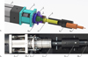Fig. 4 a. Exploded view of the PRSM traction test bench. 1: Electric jack. 2: Adaptor between jack piston and PRSM screw. 3: PRSM. 4: Adaptor between PRMS nut and Force sensor. 5: rigid frame between force sensor and Jack body. 6a: Optical displacement sensor. 6b: Force sensor. 7: Tightening and counter‐rotating elements for prestress. 8: Optical sensor aligner. b. Top view of the test bench.

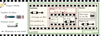Fig. 5 Automated experimental procedure for minimal human operations. Human operates only for PRSM preparation and test bench mounting. The procedure is repeated nrepetition times. First: initialisation, measuring prestress F0 and initial position d0. Second: while loop with electric jack actuation and recording of load F and position d. Third: Finalization, with data saving and return to initial state.

3.2 Experimental results

The load‐displacement curves are shown in Figure 6 considering 8, 7, 5 and 4 rollers. The 6‐roller test was prepared but the specific carriers were broken during set‐up. The data points gathered during a single trial are plotted with the same color. The confidence interval of one (dark grey) or two (light grey) standard deviations are shown. The data points show a non linear behaviour $F\propto \Delta S_1^n$ with η > 1. A best fit of data points with a pseudo‐Hertz contact law $F=\gamma {(\Delta S_1)}^{3/2}$ (dashed line) is shown to agree with data in the tested range.

As expected, the number of rollers stiffens the mechanism as the force increases from Figure 6d (4 rollers) to Figure 5a (8 rollers). This effect is directly reported in Figure 7a, where the non‐linear stiffness constant of the mechanism γ is plotted against the number of contacts. Raw data points of tests made with 8 rollers but less contact points are reported in Appendix D.

The model predictions are shown (continuous blue line) in each subplot of Figure 5 with model deviations with 5% uncertainty on PRSM parameters in blue shadow. The present model is predictive because it has no fitting parameter.

The model follows the experimental data correctly at low forces but is less accurate for large forces. The model prediction are also fitted with a pseudo‐Hertz model $F=\gamma {(\Delta S_1)}^{3/2}$, to determine γ. γ coefficients from the model are reported in Figure 7a, to compare the model predictions to experiments. In almost all trials, the model is slightly stiffer than the experiments and some variability appears between experiments. Considering a fixed number of contacts in the mechanism nn_R, the model predicts a slightly stiffer behaviour when the contacts are shared by a larger number of rollers.

Although the model does not fit perfectly experimental data, see Section 5, it gives correct trends and magnitudes. More importantly for fatigue lifespan prediction, local loads at each thread contact are directly computed by this light model which allows the identification of critical contacts. A typical load distribution is shown in Figure 7b. The local loads are larger at the side where clamping (N₂₅) and loading (S₂₅) are applied and decreases until reaching a plateau. Roller‐screw contacts are slightly stiffer than roller‐nut contacts close to the loading side. Conversely, they are slightly softer on the other side. When clamping/loading conditions are on different sides (loading configurations B and C in Fig. 3a), the load distribution in expected to be more uniform. In the following, the scenario of clamping/loading on the same side (loading configurations A and D in Fig. 3a) is considered as a worst case scenario for fatigue lifespan.

In Figure 7b, maximal loads are larger on the roller‐screw side because contacts are less conformal than roller‐nut ones. Since the total load on threads is preserved in the mechanism, the contrary occurs on the unloaded side (S₁, N₁): minimal loads supported by roller‐nut contacts are slightly larger than for roller‐screw contacts.

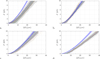Fig. 6 Force‐deformation curve of the PRSM. Experimental data points belonging to a single loading test are shown with same color. Dark grey shade : 1 σ (Experimental standard deviation). Light grey shade : 2 σ. Dashed line: best fit with 3/2 power law. Continuous line: Model prediction (No adjustable parameter). Blue shade: model deviation with 5% uncertainty on PRSM parameters. a. 8 rollers. b. 7 rollers c. 5 rollers and d. 4 rollers.

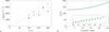Fig. 7 a. Non‐linear mechanism stiffness coefficient, γ, as a function of the number of contacts of the mechanism nnR. Model predictions (hollow symbols) are compared to experimental data points (filled symbols). Star: change of number of rollers. Circle: change of number of contacts per roller. b. Load distribution predicted by the model for F = 30 kN (8 rollers, 25 contacts per roller, $\widehat{f}$ = 150 N). Load distribution is not uniform and concentrates at the force/clamping side. Blue circle: Roller‐screw thread contact. Green diamond: Roller‐nut thread contact.

4 PRSM lifespan: modelling considering mechanism compliance and microscopic criterion

The PRSM lifespan is computed using the algorithm presented in Lepagneul et al. [19]. This algorithm is based on a microscopic criterion for crack initiation [18]. It computes the lifespan considering the material properties of steel used to manufacture the PRSM, and its geometry given in table 2. The model does not computes sliding that may vary depending on lubricant, thermal conditions and surface roughness of the mechanism parts. Rather, it outputs general lifespan maps depending on normal load and friction coefficient μ, see Figure 8.

Figure 8 shows color maps of the Dang‐Van criterion with dashed iso‐Dang‐Van criterion contours. The solid black line shows the limit of infinite fatigue lifespan. For loads on the left side of the infinite lifespan line, the predicted fatigue life is infinite. On the contrary, large loads reduces fatigue lifespan. The solid white line is the fatigue life computed for an uniform load distribution. The non‐linearity of load distribution and Dang‐Van criterion create large differences in PRSM fatigue life limits. The uniform load distribution predicts infinite fatigue lifespan limit much larger than the one computed for the compliant mechanism.

Fig. 8 Fatigue lifespan maps of the compliant PRSM a. Roller‐screw side. b. Roller‐nut side. Black line: infinite fatigue lifespan limit for a compliant mechanism. White line: infinite fatigue lifespan limit with uniform load distribution. Color map and contours show levels of Dang Van criterion.

Fig. 9 Synchronous measurement of force and displacement of the PRSM. a. 3s‐averaged load sensor signal (moving mean). Red patch indicates zone of almost nil force with fluctuations (red arrows). b. Raw displacement signal. Vertical blue arrow: clearance closing before engagement. Horizontal arrows: step size variation indicating stick‐slip behaviours or clearances in the mechanism.

5 Discussion

The PRSM fatigue lifespan depends on the compliance of the mechanism, which is difficult to compute due to the large number of threaded contacts and their nonlinear load‐displacement relationships. The modelling of compliance rely on the linearization of Hertz contact load‐displacement relation. The load distributions are similar on the roller‐nut and roller screw sides. The range of variation on the roller‐screw side is slightly larger than on the roller‐nut side. This is the consequence of a smaller contact conformity at the roller‐screw side.

More importantly, the present modelling of fatigue lifespan shows a large effect of compliance on the maximal load at infinite lifespan. It was previously shown that the roller‐screw side was the most sensitive for fatigue lifespan limit in the typical range of sliding coefficient (μ ≤ 0.1) [19]. This effect is slightly more pronounced considering compliance since larger thread forces are encountered at roller‐screw contacts.

Considering Figure 6a, model predictions are not matching perfectly experimental data points. This is due to two factors:

– The main factor is the experimental difficulty to find the beginning of a non‐linear contact. The non‐linear power law of force displacement $F=\gamma \Delta S_1^{3/2}$ starts with a horizontal tangent for $\Delta S_1=0$ meaning that a large error may occur on delta when finding the first positive force F > 0. Furthermore, despite precautions taken to pre‐stress the sensor, it still fluctuates at small forces leading to difficulties in detecting the first positive mean value as show by red arrows in Figure 9a. This could be improved by using a sensor with a smaller load range. Finally, the complexity of the mechanism, with 3D clearances, involves the stick‐slip positioning of moving element (such as rollers) during loading before complete engagement of all parts of the mechanism, see Figure 9b. This phenomenon, clearly observable on temporal measurements (horizontal arrows), creates some fluctuations on the force‐displacement curves at small loads. Despite similar observations of non‐linear behaviors, these experimental difficulties have not been reported elsewhere [9, 10, 15].

– The second factor of discrepancy lies in the model itself that predicts larger stiffness than experimentally tested. This artefact is present in every analytical modelling of PRSM stiffness [5, 8–10]. In previous models of PRSM stiffness, thread structural stiffness has been modelled as linear with annular plate models [5, 9] or more realistic triangular thread models taking into account bending, shear, root incline, root shear and radial deformation [8, 10]. This triangular beam model used by Zhang et al. [8] is said by the authors to overestimate thread deformations. As thread structural stiffness and contact stiffness are in series, the linear behaviour is expected to occur at large loads where the non‐linear contact stiffness becomes much larger than the thread structural stiffness. However, for small to moderate loads, only the non‐linear effect of the contact stiffness is expected. For the sake of simplicity and clarity, the thread structural stiffness was not considered in this model since it adds more parameters to the modelling. Furthermore, the thread geometry is more complex than a flat annular plate or even a triangular plate since roller threads are convex. The consequence of this modelling choice is that the present model only works well for small to moderate loads (F ≤ 8 kN). Nevertheless, this range of loads encloses infinite fatigue lifespan limit. At 6 kN, the approximate range of infinite lifespan, the present model underestimate deformations by 19.5% in average which is in the same range as similar modelling, 21% (at 5 kN) for [5]. Other models give directly the error in term of stiffness, 12% error in stiffness at 10 kN in [10] and finally 6.41% in stiffness in the range 0 to 10 kN in [9]. Major modelling improvement lies in the modelling of thread and global structural stiffness to take into account the linear behaviour observed at large loads and to predict the number of cycles before crack initiation by fatigue at large loads.

6 Conclusion

A comprehensive pipeline is proposed to determine the infinite lifespan loads from PRSM geometry and material parameters. The fatigue lifespan of a PRSM has been modelled considering PRSM compliance and a multiaxial fatigue criterion. The compliance modelling has been compared to experimental data and has been shown to be valid for small to moderate loads usually encountered in fatigue. The proposed modelling of PRSM stiffness is predictive because it has no fitting parameter. Differently from previous models, the proposed modelling has been made minimal to study compliance effects in the context of fatigue loading. Thus it does not consider thread structural stiffness that adds supplementary parameters which are currently not well mastered for convex‐annular‐triangular threads. Thread structural stiffness softens the mechanism at high loads.

The effect of mechanism compliance is to concentrate loads close to sides where boundary conditions are applied (load or clamping). It is shown to decrease the fatigue lifespan limit. The non‐uniform load distribution reinforces the criticality of the roller‐screw side when considering PRSM fatigue design in the range of classical lubrication (μ ≤ 0.1) .

Experimental data on thread wear and fatigue crack initiation on complete PRSMs are necessary to fully validate this model. Those experimental tests require long runs (millions of cycles) and repetition over identical mechanisms to obtain fatigue statistical results.

Funding

This work was jointly supported by ANRT (CIFRE, No. 2021/0010), Airbus Helicopters and Aix‐Marseille University.

Conflicts of interest

The authors declare that they have no known competing financial interests or personal relationships that could have appeared to influence the present work.

Data availability statement

All data generated or analyzed during this study are included in this published article.

Author contribution statement

J.L. was the main investigator. Tasks: experiment design and manufacturing, data acquisition, data treatment, modelling and manuscript writing. L.T. Tasks: data acquisition, data treatment, modelling and manuscript writing. E.M. Tasks: funding acquisition and manuscript review. J.D. Tasks: experiment design and manufacturing. J‐M.L : funding acquisition, experiment design and manufacturing, modelling and manuscript review.

References

Appendix

Appendix A: Hertz contact algorithm

Hertz contact is a well established mechanical problem. We give here a numerical recipe to compute Hertz geometry efficiently using matlab ellipke function. Equations implemented were found in [20].

We first define functions ϕ₁ and ϕ₂,

$$\begin{array}{l}{\varphi }_1(k)={\int }_0^{\infty }\frac{\text{d}u}{\sqrt{{(1+u)}^3(1/k^2+u)u}}=\frac{2k^2(kK-E/k)}{k^2-1}\hfill \\ {\varphi }_2(k)={\int }_0^{\infty }\frac{\text{d}u}{\sqrt{(1+u)(1/k^2+u{)}^{3}u}}=\frac{2k^3(E-K)}{k^2-1}\hfill \end{array}$$(A.1)

where K and E are elliptic integrals of argument 1–k²: [K,E] = ellipke(1‐k²).

We also define the geometrical parameters A and B from the principal curvatures of the two surfaces in contact and the angle β between the two frames :

$$\begin{array}{l}2(B+A)={\rho }_{11}+{\rho }_{12}+{\rho }_{21}+{\rho }_{22}\hfill \\ 2(B-A)={\left({({\rho }_{11}-{\rho }_{12})}^2+{({\rho }_{21}-{\rho }_{22})}^2+2({\rho }_{11}-{\rho }_{12})({\rho }_{21}-{\rho }_{22})cos(2\beta )\right)}^{1/2}\hfill \end{array}$$(A.2)

From these definitions, a Newton‐Raphson algorithm is implemented to find the right k of the problem by finding the root of

$$A{\varphi }_2(k)-B{\varphi }_1(k)=0$$(A.3)

From this, we determine the Hertz coefficient,

$$ɑ=\frac{\pi }{3}\frac{E}{(1-{\nu }^2)}\frac{\sqrt{{\varphi }_1(k)+{\varphi }_2(k)}}{k^{3/2}{K}^{3/2}\sqrt{{\rho }_{11}+{\rho }_{12}+{\rho }_{21}+{\rho }_{22}}}$$(A.4)

Appendix B: Linearization of Hertz contact force

The Hertz contact force‐displacement reads $x=f^{2/3}/{ɑ}^{2/3}$. Introducing the average contact force, $x={\left(\left(f-\widehat{f}\right)/\widehat{f}+1\right)}^{2/3}{\widehat{f}}^{2/3}/{ɑ}^{2/3}$ and developing the Taylor series at the first order in $\left(f-\widehat{f}\right)/\widehat{f}$ gives

$$x=\frac{1}{{ɑ}^{2/3}}{\widehat{f}}^{2/3}\left(1+\frac{2}{3}\frac{f-\widehat{f}}{\widehat{f}}\right)$$(B.1)

Rewriting this relation, one finds,

$$f=\underset{k_H}{\underbrace{\left(\frac{3}{2}{ɑ}^{2/3}{\widehat{f}}^{1/3}\right)}}x-\frac{1}{2}\widehat{f}$$(B.2)

Appendix C: Boundary conditions for different loading configurations

The following equations should be considered in replacement of equation (6) when different loading configurations are tested.

Model boundary conditions for loading configuration B shown in Figure 3a (Top‐right):

$$\begin{array}{l}{N}_1=0\hfill \\ k_N(N_n-N_{n-1}-p)+k_{NR}(R_{2n-1}-N_n)-\widehat{f}/2=0\hfill \\ k_S(S_2-S_1-p)+k_{SR}(S_1-R_2)+\widehat{f}/2=0\hfill \\ F-k_S(S_n-S_{n-1}-p)-k_{SR}(S_n-R_{2n})+\widehat{f}/2=0\hfill \end{array}$$(C.1)

Model boundary conditions for loading configuration C shown in Figure 3a (Bottom‐left):

$$\begin{array}{l}{k}_N(N_2-N_1-p)+k_{NR}(R_1-N_1)-\widehat{f}{n}_R/2=0\hfill \\ F+k_N(N_n-N_{n-1}-p)+k_{NR}(R_{2n-1}-N_n)-\widehat{f}/2=0\hfill \\ S_1=0\hfill \\ -k_S(S_n-S_{n-1}-p)-k_{SR}(S_n-R_{2n})+\widehat{f}/2=0\hfill \end{array}$$(C.2)

Model boundary conditions for loading configuration D shown in Figure 3a (Bottom‐right):

$$\begin{array}{l}F+k_N(N_2-N_1-p)+k_{NR}(R_1-N_1)-\widehat{f}{n}_R/2=0\hfill \\ k_N(N_n-N_{n-1}-p)+k_{NR}(R_{2n-1}-N_n)-\widehat{f}/2=0\hfill \\ k_S(S_2-S_1-p)+k_{SR}(S_1-R_2)+\widehat{f}/2=0\hfill \\ S_n=0\hfill \end{array}$$(C.3)

Appendix D: Tests varying thread contacts per roller

Fig. D1. Force‐deformation curve of the PRSM depending on the number of contacts per roller. Experimental data points belonging to a single loading test are shown with same color. Dark grey shade : 1 σ (Experimental standard deviation). Light grey shade : 2 σ. Dashed line: best fit with 3/2 power law. a. 8 rollers with 19 contacts per roller. b. 8 rollers with 25 contacts per roller.

Appendix E: Stiffness matrix K

Depending on the number of thread contacts per roller n, the stiffness matrix K has a size 4n × 4n. This matrix is given, in the general case by equations (4), (5) and boundary conditions (6) (or boundary conditions given in Appendix C). To exemplify its shape, we give the stiffness matrix for n = 3 thread contacts per roller with boundary conditions of equation (6):

$$K=\left(\begin{array}{cccccccccc}\hfill -k_N-k_{NR}\hfill & \hfill k_N\hfill & \hfill 0\hfill & \hfill k_{NR}\hfill & \hfill 0\hfill & \hfill 0\hfill & \hfill 0\hfill & \hfill 0\hfill & \hfill 0\hfill & \hfill 0\hfill \\ \hfill 0\hfill & \hfill 0\hfill & \hfill \hfill & \hfill \hfill & \hfill \hfill & \hfill \hfill & \hfill \hfill & \hfill \hfill & \hfill \hfill & \hfill \hfill \\ \hfill k_N\hfill & \hfill -2k_N-k_{NR}\hfill & \hfill 0\hfill & \hfill 0\hfill & \hfill k_{NR}\hfill & \hfill 0\hfill & \hfill 0\hfill & \hfill 0\hfill & \hfill 0\hfill & \hfill 0\hfill \\ \hfill 0\hfill & \hfill 0\hfill & \hfill \hfill & \hfill \hfill & \hfill \hfill & \hfill \hfill & \hfill \hfill & \hfill \hfill & \hfill \hfill & \hfill \hfill \\ \hfill 0\hfill & \hfill 0\hfill & \hfill 1\hfill & \hfill 0\hfill & \hfill 0\hfill & \hfill 0\hfill & \hfill 0\hfill & \hfill 0\hfill & \hfill 0\hfill & \hfill 0\hfill \\ \hfill 0\hfill & \hfill 0\hfill & \hfill \hfill & \hfill \hfill & \hfill \hfill & \hfill \hfill & \hfill \hfill & \hfill \hfill & \hfill \hfill & \hfill \hfill \\ \hfill k_{NR}\hfill & \hfill 0\hfill & \hfill 0\hfill & \hfill -k_R-k_{NR}\hfill & \hfill k_R\hfill & \hfill 0\hfill & \hfill 0\hfill & \hfill 0\hfill & \hfill 0\hfill & \hfill 0\hfill \\ \hfill 0\hfill & \hfill 0\hfill & \hfill \hfill & \hfill \hfill & \hfill \hfill & \hfill \hfill & \hfill \hfill & \hfill \hfill & \hfill \hfill & \hfill \hfill \\ \hfill 0\hfill & \hfill 0\hfill & \hfill 0\hfill & \hfill k_R\hfill & \hfill -2k_R-k_{SR}\hfill & \hfill k_R\hfill & \hfill 0\hfill & \hfill 0\hfill & \hfill 0\hfill & \hfill k_{SR}\hfill \\ \hfill 0\hfill & \hfill 0\hfill & \hfill \hfill & \hfill \hfill & \hfill \hfill & \hfill \hfill & \hfill \hfill & \hfill \hfill & \hfill \hfill & \hfill \hfill \\ \hfill 0\hfill & \hfill k_{NR}\hfill & \hfill 0\hfill & \hfill 0\hfill & \hfill k_R\hfill & \hfill -2k_R-k_{NR}\hfill & \hfill k_R\hfill & \hfill 0\hfill & \hfill 0\hfill & \hfill 0\hfill \\ \hfill 0\hfill & \hfill 0\hfill & \hfill \hfill & \hfill \hfill & \hfill \hfill & \hfill \hfill & \hfill \hfill & \hfill \hfill & \hfill \hfill & \hfill \hfill \\ \hfill 0\hfill & \hfill 0\hfill & \hfill 0\hfill & \hfill 0\hfill & \hfill 0\hfill & \hfill k_R\hfill & \hfill -2k_R-k_{SR}\hfill & \hfill k_R\hfill & \hfill 0\hfill & \hfill 0\hfill \\ \hfill k_{SR}\hfill & \hfill 0\hfill & \hfill \hfill & \hfill \hfill & \hfill \hfill & \hfill \hfill & \hfill \hfill & \hfill \hfill & \hfill \hfill & \hfill \hfill \\ \hfill 0\hfill & \hfill 0\hfill & \hfill k_{NR}\hfill & \hfill 0\hfill & \hfill 0\hfill & \hfill 0\hfill & \hfill k_R\hfill & \hfill -2k_R-k_{NR}\hfill & \hfill k_R\hfill & \hfill 0\hfill \\ \hfill 0\hfill & \hfill 0\hfill & \hfill \hfill & \hfill \hfill & \hfill \hfill & \hfill \hfill & \hfill \hfill & \hfill \hfill & \hfill \hfill & \hfill \hfill \\ \hfill 0\hfill & \hfill 0\hfill & \hfill 0\hfill & \hfill 0\hfill & \hfill 0\hfill & \hfill 0\hfill & \hfill 0\hfill & \hfill k_R\hfill & \hfill -k_R-k_{SR}\hfill & \hfill 0\hfill \\ \hfill 0\hfill & \hfill k_{SR}\hfill & \hfill \hfill & \hfill \hfill & \hfill \hfill & \hfill \hfill & \hfill \hfill & \hfill \hfill & \hfill \hfill & \hfill \hfill \\ \hfill 0\hfill & \hfill 0\hfill & \hfill 0\hfill & \hfill 0\hfill & \hfill k_{SR}\hfill & \hfill 0\hfill & \hfill 0\hfill & \hfill 0\hfill & \hfill 0\hfill & \hfill -k_S-k_{SR}\hfill \\ \hfill k_S\hfill & \hfill 0\hfill & \hfill \hfill & \hfill \hfill & \hfill \hfill & \hfill \hfill & \hfill \hfill & \hfill \hfill & \hfill \hfill & \hfill \hfill \\ \hfill 0\hfill & \hfill 0\hfill & \hfill 0\hfill & \hfill 0\hfill & \hfill 0\hfill & \hfill 0\hfill & \hfill k_{SR}\hfill & \hfill 0\hfill & \hfill 0\hfill & \hfill k_S\hfill \\ \hfill -2k_S-k_{SR}\hfill & \hfill 0\hfill & \hfill \hfill & \hfill \hfill & \hfill \hfill & \hfill \hfill & \hfill \hfill & \hfill \hfill & \hfill \hfill & \hfill \hfill \\ \hfill 0\hfill & \hfill 0\hfill & \hfill 0\hfill & \hfill 0\hfill & \hfill 0\hfill & \hfill 0\hfill & \hfill 0\hfill & \hfill 0\hfill & \hfill k_{SR}\hfill & \hfill 0\hfill \\ \hfill k_S\hfill & \hfill -k_S-k_{SR}\hfill & \hfill \hfill & \hfill \hfill & \hfill \hfill & \hfill \hfill & \hfill \hfill & \hfill \hfill & \hfill \hfill & \hfill \hfill \\ \hfill \hfill & \hfill \hfill & \hfill \hfill & \hfill \hfill & \hfill \hfill & \hfill \hfill & \hfill \hfill & \hfill \hfill & \hfill \hfill & \hfill \hfill \end{array}\right)$$(E.1)

All Tables

All Figures

	Fig. 1 Components of an inverted PRSM. The nut (1‐green) encloses rollers (4‐light grey) and screw (3‐blue). The rollers are placed in contact with the screw by two carriers (2‐red) which are in pivot joint with the screw and locked by two circlip rings (5‐grey).
In the text

	Fig. 2 Diagram of PRSM kinematics. a. Standard PRMS. Rollers do not translate regarding nut. b. Inverted PRSM. Rollers do not translate regarding screw. N‐green : Nut. R‐grey : Rollers. S‐blue: Screw. C‐red: Carriers. Punctual contacts are shown with arrows and circles.
In the text

Fig. 3 a. Experimental loading configurations. Green: nut. Blue: screw. A (Top‐left): External load on screw and clamped nut on same side. B (Top‐right): External load on screw and clamped nut on opposite side. C (Bottom‐left): External load on nut and clamped screw on opposite side. D (Bottom‐right): External load on nut and clamped screw on same side. b. Modelling of a compliant PRSM (configuration A) inspired from [5]. Only one equivalent roller is shown. The nut (resp. screw) has n contacts with the equivalent roller. 5 different springs are considered: bulk nut kN, bulk screw kS, bulk roller kR, roller‐screw contact kSR and roller‐nut contact kNR.

In the text

	Fig. 4 a. Exploded view of the PRSM traction test bench. 1: Electric jack. 2: Adaptor between jack piston and PRSM screw. 3: PRSM. 4: Adaptor between PRMS nut and Force sensor. 5: rigid frame between force sensor and Jack body. 6a: Optical displacement sensor. 6b: Force sensor. 7: Tightening and counter‐rotating elements for prestress. 8: Optical sensor aligner. b. Top view of the test bench.
In the text

Fig. 5 Automated experimental procedure for minimal human operations. Human operates only for PRSM preparation and test bench mounting. The procedure is repeated nrepetition times. First: initialisation, measuring prestress F0 and initial position d0. Second: while loop with electric jack actuation and recording of load F and position d. Third: Finalization, with data saving and return to initial state.

In the text

Fig. 6 Force‐deformation curve of the PRSM. Experimental data points belonging to a single loading test are shown with same color. Dark grey shade : 1 σ (Experimental standard deviation). Light grey shade : 2 σ. Dashed line: best fit with 3/2 power law. Continuous line: Model prediction (No adjustable parameter). Blue shade: model deviation with 5% uncertainty on PRSM parameters. a. 8 rollers. b. 7 rollers c. 5 rollers and d. 4 rollers.

In the text

Fig. 7 a. Non‐linear mechanism stiffness coefficient, γ, as a function of the number of contacts of the mechanism nnR. Model predictions (hollow symbols) are compared to experimental data points (filled symbols). Star: change of number of rollers. Circle: change of number of contacts per roller. b. Load distribution predicted by the model for F = 30 kN (8 rollers, 25 contacts per roller, $\widehat{f}$ = 150 N). Load distribution is not uniform and concentrates at the force/clamping side. Blue circle: Roller‐screw thread contact. Green diamond: Roller‐nut thread contact.

In the text

	Fig. 8 Fatigue lifespan maps of the compliant PRSM a. Roller‐screw side. b. Roller‐nut side. Black line: infinite fatigue lifespan limit for a compliant mechanism. White line: infinite fatigue lifespan limit with uniform load distribution. Color map and contours show levels of Dang Van criterion.
In the text

	Fig. 9 Synchronous measurement of force and displacement of the PRSM. a. 3s‐averaged load sensor signal (moving mean). Red patch indicates zone of almost nil force with fluctuations (red arrows). b. Raw displacement signal. Vertical blue arrow: clearance closing before engagement. Horizontal arrows: step size variation indicating stick‐slip behaviours or clearances in the mechanism.
In the text

	Fig. D1. Force‐deformation curve of the PRSM depending on the number of contacts per roller. Experimental data points belonging to a single loading test are shown with same color. Dark grey shade : 1 σ (Experimental standard deviation). Light grey shade : 2 σ. Dashed line: best fit with 3/2 power law. a. 8 rollers with 19 contacts per roller. b. 8 rollers with 25 contacts per roller.
In the text

References

- X. Li, G. Liu, X. Fu, S. Ma, Review on motion and load‐bearing characteristics of the planetary roller screw mechanism, Machines 10, 317 (2022) [Google Scholar]
- M.H. Jones, S.A. Velinsky, T.A. Lasky, Dynamics of the planetary roller screw mechanism, J. Mech. Robot. 8, (2016) [Google Scholar]
- S. Sandu, N. Biboulet, D. Nelias, F. Abevi, An efficient method for analyzing the roller screw thread geometry, Mech. Mach. Theory 126, 243–264 (2018) [Google Scholar]
- S. Ma, G. Liu, R. Tong, X. Zhang, A new study on the parameter relationships of planetary roller screws, Math. Probl. Eng. 2012, (2012) [Google Scholar]
- M. H. Jones, S. A. Velinsky, Stiffness of the roller screw mechanism by the direct method, Mech. Based Des. Struct. Mach. 42, 17–34 (2014) [Google Scholar]
- J. Ry´s, F. Lisowski, The computational model of the load distribution between elements in a planetary roller screw, J. Theor. Appl. Mech. 52, 699–705 (2014) [Google Scholar]
- X. Du, B. Chen, Z. Zheng, Investigation on mechanical behavior of planetary roller screw mechanism with the effects of external loads and machining errors, Tribol. Int. 154, 106689 (2021) [Google Scholar]
- W. Zhang, G. Liu, R. Tong, S. Ma, Load distribution of planetary roller screw mechanism and its improvement approach, Proc. Inst. Mech. Eng. Part C: J. Mech. Eng. Sci. 230, 3304–3318 (2016) [Google Scholar]
- J. Guo, H. Peng, H. Huang, Z. Liu, Y. Huang, W. Ding, Analytical and experimental of planetary roller screw axial stiffness, in: 2017 IEEE International Conference on Mechatronics and Automation (ICMA), IEEE, 2017, pp. 752–757 [Google Scholar]
- S. Ma, G. Wu, J. Zhang, G. Liu, Experimental research on static stiffness of the planetary roller screw mechanism, in: MATEC Web of Conferences, EDP Sciences, vol. 306, 2020, p. 02002 [Google Scholar]
- R. Hu, H. Liu P. Wei, X. Du, P. Zhou, C. Zhu, Investigation on load distribution among rollers of planetary roller screw mechanism considering machining errors: analytical calculation and machine learning approach, Mech. Mach. Theory 185, 105322 (2023) [Google Scholar]
- F. Abevi, A. Daidie, M. Chaussumier, M. Sartor, Static load distribution and axial stiffness in a planetary roller screw mechanism, J. Mech. Des. 138, (2016) [Google Scholar]
- W. Zhang, G. Liu, S. Ma, R. Tong, Load distribution over threads of planetary roller screw mechanism with pitch deviation, Proc. Inst. Mech. Eng. Part C: J. Mech. Eng. Sci. 233, 4653–4666 (2019) [Google Scholar]
- J. Otsuka, T. Osawa, S. Fukada, A study on the planetary roller screw (comparison of static stiffness and vibration characteristics with those of the ball screw), Bull. Jpn. Soc. Precis. Eng. 23, 217–223 (1989) [Google Scholar]
- F. Abevi, A. Daidie, M. Chaussumier, S. Orieux, Static analysis of an inverted planetary roller screw mechanism, J. Mech. Robot. 8, (2016) [Google Scholar]
- J. Meng, X. Du, Y. Li, P. Chen, F. Xia, L. Wan, A multiscale accuracy degradation prediction method of planetary roller screw mechanism based on fractal theory considering thread surface roughness, Fractal Fract. 5, 237 (2021) [Google Scholar]
- G. Auregan, V. Fridrici, P. Kapsa, F. Rodrigues, Experimental simulation of rolling–sliding contact for application to planetary roller screw mechanism, Wear 332, 1176–1184 (2015) [Google Scholar]
- K. Dang‐Van, Introduction to fatigue analysis in mechanical design by the multiscale approach, in: High‐cycle Metal Fatigue, Springer, 1999, pp. 57–88 [Google Scholar]
- J. Lepagneul, L. Tadrist, J.‐M. Sprauel, J.‐M. Linares, Fatigue lifespan of a planetary roller‐screw mechanism, Mech. Mach. Theory 172, 104769 (2022) [Google Scholar]
- W. Goldsmith, Impact. The Theory and Physical Behaviour of Colliding Solids, Courier Corporation, 2001 [Google Scholar]
Cite this article as: J. Lepagneul, L. Tadrist , E. Mermoz, J. Diperi, J.-M. Linares, Fatigue lifespan of compliant planetary roller screws: Multiscale modelling and stiffness measurements, Mechanics & Industry 27, 3 (2026), https://doi.org/10.1051/meca/2025030