| Issue |
Mechanics & Industry
Volume 26, 2025
|
|
|---|---|---|
| Article Number | 21 | |
| Number of page(s) | 26 | |
| DOI | https://doi.org/10.1051/meca/2025013 | |
| Published online | 09 June 2025 | |
Original Article
Identification of key parameter influence on efficiency of chain drive for track cycling − Preliminary results
INSA Lyon, CNRS, LaMCoS, UMR5259, 69621 Villeurbanne, France
* e-mail: This email address is being protected from spambots. You need JavaScript enabled to view it.
Received:
20
December
2024
Accepted:
17
April
2025
Abstract
The presented paper investigates the efficiency of chain drive transmissions in track cycling, where performance optimization is critical as a win or loss between athletes is often decided in a matter of 1/100 seconds. A 2D quasi-static model (Chain Drive Efficiency Model, CDEM) was previously developed. It includes first a simulation of the global kinematics and then uses the roller movement along tooth profiles as well as the relative movement of chains part to calculate the efficiency. A dedicated experimental test rig was also designed to reproduce the chain transmission track cycling conditions. The test rig features two instrumented shafts with torque transducers, enabling efficiency measurements under distinct loading conditions representative of endurance and sprint races. Results from both the model and test rig confirm the significant influence of chain tension and sprocket tooth number on efficiency, while misalignment showed negligible effects. Lubrication tests revealed that solid wax-based lubricants provide notable performance improvements. At the contact scale, the study compared industrial tooth profiles to newly proposed cycling-specific profiles. The CDEM predictions, consistent with experimental data, identified meshing losses as the primary source of dissipation, while roller-related losses were negligible. These findings provide insights for optimizing track cycling chain transmissions and highlight the potential of localized improvements, including lubricant choice and tooth profile design.
Key words: Efficiency / track cycling / 2D quasi-static model / track cycling test bench
These authors contributed equally to this work.
© G. Lanaspeze et al., Published by EDP Sciences 2025
 This is an Open Access article distributed under the terms of the Creative Commons Attribution License (https://creativecommons.org/licenses/by/4.0), which permits unrestricted use, distribution, and reproduction in any medium, provided the original work is properly cited.
Nomenclature
CI,II: Applied torque [N.m]
D: Diameter [m]
Eo: Experimental offset [W]
K, K ': Constants for calculation of ϕtp (specific to each tooth profile family) [rad/deg]
L: Distance between the axes of the driving and driven sprockets [m]
mlink: Mass of the link [g]
n: Number of chain links [−]
N: Equivalent number of links [−]
P: Roller/sprocket contact load [N]
ΔP: Relative loss of two transmission configurations [W]
R: Radius [m]
slack: Mid-span movement as a fraction of L [−]
T: Chain tension [N]
Ts,j: Slack tension for sprocket j [N]
Tp: Temperature for experimental measurements [deg]
 : Acquisition temperature [rad]
Z: Number of teeth [−]
αI,II: Angular pitch of the sprocket [rad]
α* : Angle between two consecutive links [rad]
αs,t,j: Angle between a chain strand and the closest link with both rollers contacting sprocket j [rad]
βI,II: Angle deviation of the concerned sprocket [rad]
δ: Friction correction angle [rad]
|δ (∞) |: Correction angle outside [rad]
ΔP: Relative losses of the transmission [W]
ΔY: Vertical distance between the axes of the driving and driven sprockets [m]
η: Chain drive efficiency [−]
κ: Angle between the preceding link and local x axis [rad]
 : Friction coefficient at interface [−]
ν: Angle between the following link and local x axis [rad]
ϕ: Roller contact angle [rad]
ρ: Alignment deviation of the rear cog with respect to the chainring [m]
s: Curvilinear abscissa of roller [m]
θ: Angle for the profile definition [rad]
ζ: Driving sprocket rotation angle [rad]
Subscripts
A, B: Relative to kinematic cases A and B (used in CDEM)
i: Link index
I: For the driving sprocket/chainring
II: For the driven sprocket/rear cog
br: Relative to Bush/Roller chain interface
bush: Relative to bush
curve: Relative to curvature
pb: Relative to Pin/Bush chain interface
pin: Relative to pin
profile: Relative to the chosen tooth profile
ptich: Relative to sprocket pitch
ref: Relative to reference transmission
roller: Relative to roller
rp: Relative to Roller/Profile interface
s: Attribute of the slack chain strand
t: Attribute of the tight chain strand
tb: Relative to tooth bottom
tip: Relative to tooth tip
tp: Attribute of the roller location transition points
Superscripts
k: Drive sub-position for efficiency calculation.
1 Introduction
The chain drive transmission conveys the power between the cyclist and the real wheel. Track cycling bicycles use drive with no derailleur, no freewheel and fixed gear ratio (single speed). The variety of races (sprint to endurance) induces the transmission working conditions to range up to 130 rpm and 300 N m. Final time differences between athletes are usually very close (1/100 seconds for the men's sprint in Tokyo 2021 Olympic games). These reduced gaps justify the interest of chain drive power loss optimization as little improvements can decide the race winner hence justifying the need for accurate efficiency prediction.
Binder [1] proposed a model for industrial chain transmissions that considered the dependency between the rotation of the driving and driven sprockets using a four-bar mechanism. Thus, the strand tip positions move along the pitch circles, making it possible to model the polygonal effect and losses due to link meshing. He proposed expressions for power loss and introduced a distinction between pin and bush articulations each producing different power losses. In the 1980s, Naji and Marshek produced numerous studies aimed at improving the first approach introduced by Binder. They presented measurements of link tensions performed using an instrumented link [2,3]. Using weights to prescribe strand tension, several tension ratios Ts/Tt were tested. Due to the constraints of the experimental apparatus, measurements were carried out at quasi-static speed. It was shown that, for the loads explored (up to 850 N), the evolution of relative tension does not depend on the magnitude of absolute tension. Driving and driven sprockets were studied and differences in load evolutions were reported.
Kidd studied the efficiency of chain drives applied to road bicycles [4]. Experimental measurements were carried out to assess the effect of various parameters (lubricant, input power, sprocket size, etc.). It was shown that the derailleur system is responsible for a large share of the power losses for a road bike drive. The results show efficiencies between 95 and 98.5% for drives with a derailleur while 99% is reached for simple two-sprocket drives without a derailleur. The results showed that drive efficiency (with and without a derailleur) rises with increasing input power. As the measurements were carried out at constant speed, higher input powers were achieved by increasing the transmitted torques. This increase in drive efficiency was attributed to a decrease of the proportional contribution of slack strand meshing losses. Indeed, increasing the applied torque mostly increases the tight strand tension while maintaining the slack one constant. Therefore, the relative contribution of the slack strand decreases as the input power increases, resulting in higher efficiency. This effect is particularly visible in the presence of a derailleur system. Indeed, this system applies significant tension in the slack strand and adds articulation points at both idler sprockets. A linear relation between reciprocal tight strand tension and chain drive efficiency was proposed on the basis of the results presented. Smaller reciprocal tensions, associated with higher torques, tight strand tensions, and power, resulted in higher drive efficiencies. The effect of the number of sprocket teeth was also tested and the results showed higher efficiency for drives with larger sprockets. At the same time, Spicer et al. [5] also studied bicycle chain drives. Experimental measurements were carried out using a test rig dedicated to road bike drives. The results confirmed the linear relation between reciprocal tight strand tension and drive efficiency. However, the efficiencies measured by Spicer et al. [5] were significantly lower than those of Kidd [4]. Efficiencies fell to about 85% whereas Kidd reported efficiencies systematically above 90%. The interest of bigger sprockets was also reported experimentally.
All the experimental studies presented by Kidd [4], Spicer et al. [5], Lodge & Burgess [6], Zhang & Tak [7] and Sgamma et al. [8] were based on test rigs reproducing the architecture of a usual chain drive. These test rigs had two shafts, for the driving and driven sprockets. These shafts were instrumented to measure torque and rotational speed and ultimately calculate drive efficiency. The advantage of this approach is its similarity to the real application. Measurements can be carried out for instance at fixed torque and/or rotational speed, for various sprockets, etc. The potential addition of a derailleur system is also facilitated by the architecture. However, the main drawback of this approach lies in the measurement uncertainties. Indeed, chain drives are very efficient mechanisms (about 98% for two sprocket drives [6]). Therefore, any test rig must have high accuracy to measure potential variations between drive configurations. Moreover, chain drives can transmit considerable powers (up to 1600 W for track cycling). Therefore, expensive sensors are usually required to match the required accuracy. To get round this challenge, alterative test rigs have been proposed.
Egorov et al. [9] proposed to measure the deceleration of the drive. Providing that the inertias of both shafts are well known beforehand, the deceleration time allows measuring drive efficiency with high precision. The disadvantage of this architecture is that the efficiency obtained represents an average over the entire deceleration. Therefore, it does not allow assessing the efficiency for fixed conditions (e.g., fixed torque or rotational speed). Wragge-Morley et al. [10] proposed to build a pendulum with a chain drive. Measuring the oscillation decay characterizes the dissipations occurring in the drive. This architecture reduces uncertainties [10] as time decay can be measured more easily and with better accuracy compared to torque. However, as with the inertia-based measurement [9], such a test rig does not enable easily testing drive efficiency in fixed conditions. Moreover, any change of the sprocket tested might be difficult.
More recently, Lanaspeze et al. [11,12] have developed a quasi-static model for calculating the efficiency of chain transmission of track cycles. This model includes the calculation of the general kinematics of the chain as well as the movement of the roller along the tooth profile. It is therefore able to include this movement in the efficiency predictions. Comparison with the Lodge and Burgess model [6] and experimental results on an industrial drive have shown the value of this new model for accurate efficiency predictions, particularly at low torques.
The aim of this article is to identify and study the influence of the track cycling chain transmission key parameters on its efficiency. To this end, two ways are chosen. A dedicated test rig is built to reproduce a cycling transmission on a track (chainring, rear sprocket and chains. Its results will be compared to the 2D quasi-static model built for the study of the cycling transmission [12]. Together, they allow the study of both systems scaled transmission and contact parameter influence on the efficiency and to start the optimization of track cycling transmissions.
2 Setup presentation
2.1 Model presentation, from [12]
The Chain Drive Efficiency Model (CDEM) was introduced from [12]. It assumes that all bodies are rigid, that due to the lightweight chains, no inertia effects intervene and that the main mechanics can be modelled in a planar model. The global kinematics is considered independent from the loads and only the global motions of the bodies are modelled. The clearance between the roller and the tooth profile is neglected. The tight strand is assumed to be straight and the tension is the same for all the included links. A chord model, which includes effect of gravity, is used for the slack strand (based on [6,13]). From there, the full transmission kinematics is solved by a step-by-step algorithm ([11], Fig. 1 from [12]).
The angular sectors (assumed identical) are defined as a piecewise curve where each portion is either a circle arc or a straight line. From there, knowing the location of one roller on its profile, the adjacent one can be calculated as the concurrent point between the roller trajectory and the chain pitch distance from the previous roller. Depending on the position of each roller along its corresponding tooth profile, the relative position of consecutive links is not the same. These positions however permit the calculation of the loading condition of each link. The effect of gravity is neglected with respect to the other forces. Therefore, a chain articulation with its roller in contact with a sprocket is subjected to three external forces (Ti, the tension force in the preceding link, Ti+1, the tension force in the following link andPi, the total contact force between the roller of articulation i and its corresponding tooth profile). The three forces are concurrent at the roller centre; therefore, the torque equilibrium is always verified. The moment induced by the tangential friction force is neglected. The equilibrium equation can therefore be written in the following form:
 (1)
(1)
With ϕi : Roller i (roller/link index) contact angle; δ: Correction factor of the angle ϕi for effect of friction, based on µs representing the static friction coefficient at the roller/tooth interface [14];  : angle between two consecutive links.
Finally, the ratio between the tight (Tt) and slack (Ts) strand tensions is expressed in equation (2) considering the consecutive equilibrium of all the articulations in contact with the sprocket.
 (2)
(2)
With n : number of links.
The efficiency is calculated for each chain drive articulation (i.e., set of pin, bush and roller, Fig. 2). From the angles defined in the companion article, the efficiency of each articulation can be separated in two extreme cases A and B (respectively no sliding and pure sliding) for which the tangential load can be calculated according to Coulomb law. Those calculations lead to the expressions Table 1 for the dissipated work at each interface between two sub-positions (k and k + 1) of the model.
From those results, the efficiency of the drive can be calculated. The dissipated works depend on the kinematic case considered (case A or B). Therefore, two efficiency values ηA and ηB are obtained, one for each kinematic case. The chain drive model introduced in this paper is quasi static. Therefore, its results are independent of the drive rotational speed.
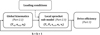 |
Fig. 1 Global CDEM algorithm, from [12]. With Ts,j:, αs,t,j:, nj, global variables, respectively slack tension, angle between a chain strand and the closest link with both rollers contacting spocket j (with j = I, II for chainring and rear cog) and contact number of rollers Ti, Pi, sc,r,i, κi, νi local variables, respectively link tension, roller contact force, curvilinear abscissa of roller, angle between the direction of the preceding link and the local x axis and the angle between the direction of the following link and the local x axis et k drive sub-position for efficiency calculation. |
2.2 Track cycling test bench description
A test rig dedicated to measurements of track cycling drive efficiency was developed at the LaMCoS1 laboratory (see Fig. 3a). This test rig mimics a track cycling drive. Two shafts, representing the chainring and rear cog axes are instrumented with torque transducers measuring both torque and rotational speed. No derailleur system is present. Rotational speed is imposed on Shaft 1 while resistive torque is imposed on Shaft 2 (see Fig. 3b). The power is delivered and absorbed by two servo motors. Bearings are mounted between the drive and torque transducers. Consequently, comparing the power between the two shafts gives a measure of the efficiency of the tested drive plus the losses of the bearings and torque transducers.
The experimental study includes transmissions with different sprockets, chainrings or lubricants, but also different settings: tension or chainline. The tests are performed at constant speed and resistive torque.
Every test session follows the protocol (Fig. 4):
After warming up the test rig for 10 min, the zero deviation (offset) of the torquemeters is measured.
The first configuration is mounted on the test rig. It then runs for 15 min, with an acquisition at 5, 10, 15 min. The offsets of the torquemeters are measured again at the end.
ii, is repeated with the other configurations to be tested.
Each configuration is tested several times to reduce uncertainties.
Measurements of the offset Eo show that it is linearly dependent of the torquemeter temperature. Therefore, the acquisitions are post-treated to correct the measured torque of both shafts. It is linearly interpolated based on the temperature and the offset before and after the test session.  and
and  for temperature,
  and
and  for offset of the torquemeters on the acquisition measure, with the temperature during the acquisition
  (see Eq. (3)).
 (3)
(3)
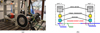 |
Fig. 3 Track cycling efficiency test rig (a) general view (b) diagram. |
 |
Fig. 4 Illustration of the test protocol. |
2.3 Test case definition
All the configurations are compared with a reference one: track chain, chainring and sprocket of width 1/8” and a 1/2” pitch. These components are from well-known manufacturers for high level track cycling. There are called “Reference” in the rest of this paper. When not indicated, the chain lubricant is the manufacturer one, already present. No special coating is applied on the chain and sprockets surfaces.
All the comparisons are performed using track cycling chains with their original lubricant. The characteristics of the chains used are given in Table 2.
The influence of chain tension was tested for two loading conditions (denoted LC1 and LC2) described in Table 3. The first condition (LC1) shows reduced output torque (on Shaft 2) compared to LC2. LC2 also exhibits higher rotation speeds. These conditions have been chosen to be representative of extreme track cycling applications. LC2 is representative of a high intensity sprint while LC1 mimics endurance races.
Track cycling chain dimensions for validation purpose.
Tested loading conditions for comparison between experiments and model results.
3 Analyses at the system scale
3.1 Influence of the tension
The chain tension is set by moving the center distance between the two shafts. On track bicycle as on the test rig, it is done by moving the sprocket shaft horizontally. A representation of the tension is obtained by measuring the tight strand deflection. On the test rig, it is evaluated using a weight of 1 kg applied on the middle of the upper strand. The obtained value is the tight strand deflection. The tight strand deflection is the deflection compared to the straight-line linking sprocket tangent (see Fig. 5a). The resulting centre distance L is measured as shown in Figure 5b.
To perform comparisons with these experimental results, the CDEM is tested with the parameters given in Table 4. The Reference tooth profile geometry is used for all calculations. The values of L are chosen to obtain slack strand looseness ranging from 2% (tightest setting) to 20% (loosest setting). The range of explored tensions should be wider with the model than with the test rig. Indeed, slack = 2% roughly corresponds to a tight strand deflection of 2/100 × 383 × 1/2 = 3.8mm and slack = 20% should correspond to about 39mm (range to be compared with from 5 to 30mm with the test rig). However, this comparison between the measured deflection and the computed one can only be carried out for an order of magnitude. Indeed, the chain drive model neglects roller/profile clearance for global kinematics [12]. Therefore, its centre distance predictions are underestimated as roller/profile but also chain articulation clearances must be overcome to reach the required tension (these clearances are neglected in the model, see [12]). Therefore, the centre distances L predicted by the model are systematically lower than that applied on the test rig to obtain a similar tension setting.
Figure 6 illustrates the two extreme tension settings (i.e., tight strand deflections of 5 and 30 mm) using the drive arrangements predicted by the CDEM. One can note that the number of links in contact with the chainring decreases as the slack strand became looser (strand tips are shown in red).
The total losses measured by the test rig (losses from the drive and from the bearings) are presented in Figure 7. The tests were performed by sessions of 25 minutes with efficiency measurements at 5, 15 and 25 min, according to protocol defined in Figure 4. Each tension setting (i.e., tight strand deflection value) was tested during 6 sessions (i.e., 18 efficiency measurements). The minimal and maximal values as well as the standard deviation are also represented in Figure 7.
Tighter settings correspond to small tight strand deflections (left of the graph) while looser settings are on the right of the graph. For LC1, as expected, the total losses decrease as the tension setting became looser. Starting from 15 mm of tight strand deflection, the losses seem to reach a plateau where additional strand looseness does not result in less dissipation. On the contrary, between 5 and 10 mm deflection, the effect of the tension setting is more significant. Between the tightest and the loosest settings, the mean difference in power losses reaches ΔP = 0.89 W. For LC2 however, no significant effect is visible. For LC2 the standard deviation reaches about 1.5 W. The consequence of these efficiency values in terms of power dissipated by the chain drive are represented in Figure 8. Power loss differences between the tightest (slack = 2%) and the loosest (slack = 20%) settings ΔP are given.
According to the CDEM predictions (Tab. 5), losses are reduced for higher slack settings for both loading conditions (LC1 and LC2). Consistently with the experimental measurements, the dissipated losses tend to an asymptote for high slack settings. The strong reduction in losses measured by the test rig between 5 and 10mm deflection (see Fig. 7) is also visible between slack=2 and ≈6% in the model predictions (see Fig. 8). A difference of ΔP=1.4W is predicted by the model between the two extreme tension settings (i.e., slack = 2% and 20%). This difference is consistent with the measurement of 0.89W by the test rig. Moreover, the interval of tension setting explored by the model is probably wider than that explored with the test rig. This wider interval will tend to increase the predicted ΔP, especially at low slack settings (high tension) where small looseness variations cause high efficiency differences. For LC2, due to the higher transmitted power, the model predicts a difference of dissipated power of 2.37 W between the two extreme settings. This difference was not observed in the test rig results. However, the predictions of the CDEM are within the order of magnitude of the measurement dispersions. Therefore, the predicted relation between the tension setting and drive losses is difficult to measure with the sensors available.
Although the prediction of ΔP is higher for LC2 than for LC1, its relative influence compared to the losses of the drive is significantly lower. ΔP reaches 1.4 W compared to a loss of about 5.5 W for LC1. For LC2, the drive losses represent about 16 W with ΔP = 2.37 W for LC2. Therefore, the influence of the slack setting decreases as torque increases. For LC1, CDEM predictions and experimental results agree on the asymptotical relation between tension setting and losses. Differences of dissipated power between the two extreme settings ΔP are also in accordance. The model prediction is higher but this difference could be explained by the difficulties of representing the same tension setting for both the test rig and the numerical model. For LC2 no significant results were observed in the test rig measurements. However, CDEM predictions show that the effect should lie within the test rig uncertainties. Indeed, the dispersion of the experimental results increases with the power transmitted.
 |
Fig. 5 Measurement of (a) tight strand deflection and (b) centre distance L. |
Transmission parameters for the tension influence study.
 |
Fig. 6 60|15 drives (a) slack=2% (b) slack=20%. Both figures have the same scale. |
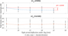 |
Fig. 7 Total power losses measured by the test rig for tension settings. |
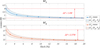 |
Fig. 8 Influence of tension setting: CDEM predictions. |
Comparison of the ΔP asymptote predictions between test rig measurements and CDEM predictions for LC1 and LC2.
3.2 Tooth number
The second comparison between the CDEM prediction and the test rig results is carried out considering efficiency results for different numbers of teeth. Two configurations with the same gear ratio ZI/ZII = 4 are considered: ZI|ZII = 60|15 and 52|13 (see Tab. 6). Sprocket size differences can be appreciated in Figure 9 showing drive arrangements predicted by the CDEM. The comparison between the two drives is carried out for the two loading conditions given in Table 3. A chainring and a rear cog both corresponding to the Reference tooth profile were used for all the tests. The test rig centre distance L is chosen to obtain a tension setting representative of a typical track cycling drive (tight strand deflexion under 1 kg mass of ≈20 mm). The resulting centre distances varied from 381 to 386 mm. It can be noted that the tight strand deflection considered lies at the plateau where differences in slack settings have minimal consequences on efficiency (see Fig. 7). Chains of 100 and 94 links were used for the 60|15 and 52|13 drives, respectively.
The total losses (drive + bearings) measured by the test rig are presented in Figure 10a. The mean values are given with the minimal and maximal measurements and the standard deviation. As for the previous case, the results were obtained by performing 25-minute tests of each configuration with efficiency measurements at 5, 15 and 25 minutes. 3 and 4 sessions were performed for 52|13 and 60|15 at LC1, respectively (corresponding to a total of 9 and 12 measurements, respectively). For LC2, 8 sessions were performed for both configurations (24 measurements) in order to reduce uncertainties.
For both loading conditions, the predicted efficiencies are higher for the 60|15 drive. Moreover, efficiencies are also higher for LC2 (with more torque) than for LC1 and the interval [ηA, ηB] between efficiency calculated in case A and B (part 2.1, Tab. 1) is reduced (see Fig. 10b). Consequently, in accordance with the test rig results, loss predictions are higher for the 52|13 drive. Loss differences ΔP measured by the test rig and calculated with the CDEM are given in Table 7.
Test rig results and CDEM predictions agreed that the 60|15 drive is always more efficient than the 52|13. Moreover, the orders of magnitude of the ΔP are similar for the CDEM and the test rig. However, model predictions in terms of ΔP are lower than test rig measurements. This is particularly true for LC1 where the prediction is about half the measured value. For LC2, the model prediction is within the test rig error bars (see Fig. 10.a).
It is possible that the slack settings used for the CDEM were looser than the test rig ones. Indeed, as mentioned above, tension settings are difficult to compare between the CDEM and the test rig. This could explain the lower ΔP predictions as increasing the slack strand tension (i.e., reducing the strand deflection) would automatically increase the radial loss inside the bearings and therefore the differences between 52|13 and 60|15 (see Fig. 7). As this effect decreases with increasing torque [12] this could explain why the CDEM predictions for ΔP are better for LC2 than for LC1. However, the slack setting tested should lie at the plateau where this effect should not be very significant. It is also possible that the assumed friction coefficients (0.11 for all interfaces) are too low and that more dissipative contacts occur for the drive tested, resulting in higher ΔP.
Nevertheless, test rig measurements and model predictions both agreed that bigger sprockets exhibit higher efficiency. This result is consistent with the literature as it has already been reported both experimentally [4,6,15] and by models [5,6,15,16]. Moreover, the order of magnitudes obtained for loss differences ΔP are consistent between test rig measurements and model predictions, suggesting that no important phenomenon has been neglected.
Transmission parameters depending on tooth number.
 |
Fig. 9 (a) 60|15 and (b) 53|13 drive, both with a looseness setting of slack=11%. Both figures have the same scale. |
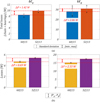 |
Fig. 10 Total power losses measured by (a) the test rig and (b) the CDEM for 60|15 and 52|13 drives for both Loading Conditions (LC1 and LC2). |
Comparison of ΔP between experimental measurements and model predictions for different sprocket sizes.
3.3 Alignment
For track cycling applications, the transmission is supposed to be aligned, the line formed by the chainring and the sprocket is called the chainline (see Fig. 11a). But as the chainline depends on the thickness of several components (frame, rear wheel, sprocket, crankset and chainring), chain offset conditions can be encountered because of different manufacturer standards (see Fig. 11b). The frame deformation can disturb the chainline, essentially when the athlete is at full power (see Fig. 11c). Another misalignment source can be the setting of the rear wheel, that is moved along a slide joint to enable chain tension setting. Because of the clearance of this slide, the rear wheel axle can be misaligned (see Fig. 11d).
Configurations noted (a), (b) and (c) in Figure 11 have been tested on the test rig. Configuration (d) has not been tested because it would require big modification of the test rig. It is assumed that the results would be similar to the configuration (c). Values for the offset of the transmission were estimated to ρ = 4mm with the bike frame manufacturer. The deformation of the frame was measured at βI = 0.3° with a load corresponding to a top-level athlete at full power. These misalignments were tested on the test rig to understand if these issues can affect the transmission efficiency. The results are plotted relatively to a well aligned transmission on Figure 12. It can be seen that the alignment has a negligible impact, hence validating the use of the 2D hypothesis in the CDEM [12].
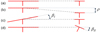 |
Fig. 11 Transmission alignment scheme. |
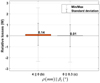 |
Fig. 12 Alignment results, Relative losses (W) compared to a well aligned transmission (a). |
3.4 Lubrication
There are hundreds of bicycle chain lubricant references available commercially. Each one claims different qualities: durability, efficiency, resistance to the humidity or to the mud, application easiness. In our case, because track cycling is practiced indoor and the races are relatively short (less than an hour), the main goal is to improve the drive efficiency of the transmission.
Power losses come from different sources [5,6,11]:
roller friction on the sprocket;
meshing loss due to the movement of the chain articulations.
Knowing that a significant part of the power losses come from meshing, the lubricant must limit the frictional forces, but also penetrate in the small gaps between the different parts of the chains. Before lubricant application, the chains are cleaned with three baths of 30 min at 65 °C in an ultrasonic cleaner. First with white spirit, then with an aqueous degreaser and finally with an ethanol bath. Once the chains are cleaned and dried, each lubricant is applied according to the manufacturer protocol. 7 lubricants are tested, compared to the manufacturer one. Lubricants DL1 and DL2 are dry lubricants, they are composed of oil and solvents. Lubricants DW1, DW2 and DW3 are liquid wax based lubricants (drip wax), they are composed of wax and solvents. SW1 and SW2 are solid wax lubricants, that need to be melted to be applied on the chain. They then solidify again inside the contact when rested after application. The transmission operation most likely melt them again and make them fluids able to separate the contact surfaces.
From Figure 13 results, it can be seen that the dry lubricants are not very efficient (DL1, DL2). For the drip wax lubricants (DW1, DW2, DW3), the conclusion is not clear, DW1 is the less efficient tested, while DW2 is one of the best. For the dry lubes and the drip waxes, it is difficult to know if the differences come from the oil or wax itself or of the solvent that pushes the lubricant to penetrate the chain. Solid wax-based lubricants are the most effective ones. the advantage compared to manufacturer lubricant is about 2W, for an input power of 490W.
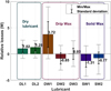 |
Fig. 13 Lubricants results, Relative losses (W) compared to manufacturer lubricant. |
4 Analyses at the contact scale
4.1 Tooth profile definition, example with ISO and ASA standard
To treat local aspects, i.e. roller displacement on tooth profile, Kim and Johnson [17] introduced the notion of the roller location characteristic curve. This curve represents the location of a given roller as a function of the location of the previous one (i.e., γi+1 as a function of γi).
Figure 14a shows roller location (parameter ξ) characteristic curves calculated by Kim and Johnson in [17]. Figure 14b shows the same curves (with parameter γ) using the CDEM. The curves are plotted for ASA profiles with Z = 12, 24 and 36. The sprocket pitch is p = 1/2'' = 12.7mm and the roller diameter is Droller = 8.51mm. The dimensions for the ASA profile are calculated according to the standard given in [1,17,18] (see Appendix A). Kim & Johnson's curves are given for coordinates ξ. It is equivalent to γ but ranges between [− 4, 4] instead of [0, 8] for the ASA profile (Fig. 15).
Figure 14 shows that the curves obtained are identical between literature and CDEM for all numbers of teeth tested, therefore validating the procedure presented. All the curves are symmetric with respect to the line y = −x consistently with the profile symmetry. Their shape is modified with the number of teeth Z. The smaller the number of teeth, the greater the deviation from the first bisector. Consequently, it takes fewer rollers to cross the zone between the transition points  ) for small Z. The transition points are the intersections with the first bisector y = x . The transition point B (i.e.
  ) lies at the at the tight side of the profile while transition point A (i.e.
  ) lies at the slack one. The transition points correspond to stable roller locations. Therefore, if roller i lies at a transition point, all the rollers will also lie at this point (following and preceding). Also, starting from the same γ beyond the transition points (i.e.,
  ), it takes fewer rollers for a small number of teeth before skipping a tooth than for a higher number. However, one cannot directly conclude that sprockets with small number of teeth will result in easier chain drop. Indeed, the link angles (e.g., α* and ϕ) and therefore the implications in terms of load calculation are different depending on Z.
It is important to remember the general dynamics of roller location. It was demonstrated by Kim & Johnson in [17] that rollers marking the transition with the tight strand always contact the tooth profile close to the transition point B (tpB). Then, depending on the loading conditions, the contact happens before or after tpB. Consequently, rollers tend to cross the profile going toward transition point A (tpA) or tend to climb the tooth flank with a high risk of chain drop. Therefore, roller location always starts at the transition point tpB (or simply tp). An example of typical roller location evolution for the ASA profile is given in Figure 16a.
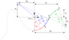
Extending the analysis, comparison of the three industrial profiles is presented in Figure 17. Markers are set at the boundary points between the curve portions in Figure 14. Transition points of each profile are indicated. The geometry of NFmin,max are the two extremes of ISO 606 [19]. This standard covers a variety of geometries with a limited number of parameters (see full definition in Appendix B).
In the local coordinate system view (Fig. 17a), the differences of tooth bottom radius (Rtb) can be appreciated. The NFminprofile is that with the smallest clearance with the roller. Along the tooth flank, the NFmin profile exhibits the steepest slopes while the NFmax has the shallowest. The slope of the profile flank does not significantly vary for the NF profiles as it is defined by a circle with a large radius (compared to the other dimensions). The ASA profile slopes lie between the two preceding profiles with significant changes along the curve. Going from the transition point to the tooth tip, the slope first lies close to the NFmax one before catching up with the NFmin and finally decreasing at the topping curve (last portion of the ASA profile). One can note that the ASA profile satisfies the ISO standards as its definition always lies between the two NF ones. The positions of the transition points are not the same for each profile. However, it is interesting to note that these specific points lie almost at the borders of the tooth bottom portion (i.e., close to γ = 5 and γ = 3 for ASA and NF profiles, respectively, see Appendix A and B). The different tip diameters can be appreciated in the global view (Fig. 17b). However, this parameter will have limited influence on the profile properties due to the transition point locations.
For the loading conditions explored in the previous part, and for both driving and driven sprockets, the rollers first lie at the tp before starting to cross the profile at different instants depending on the tooth profile (i.e., ASA, NFmax and NFmin), loading conditions, etc. Similarities have been observed in the differences between tooth profiles and between driving and driven sprockets, suggesting that the same phenomenon could explain both. Figure 18 shows plots of the pressure angle ϕi for the driving and driven sprocket (at CI = 50N . m).
The evolution of ϕi (Fig. 18) is consistent with the roller location variations. Indeed, the pressure angle depends on the directions of the previous link and profile normal at the roller/profile contact point [12]. When the rollers lie at the transition point, both directions are almost unchanged. Consequently, the pressure angle ϕi obtained is also constant. As soon as the roller starts crossing the tooth profile, the normal direction changes and the pressure angle increases. When the profile is entirely crossed (e.g., for NFmin driven sprocket) the pressure angle stabilises at a new plateau as the roller reaches the second transition point tpA. The link meshing is visible between ζ/ α = 0 and 1 where an initial decrease occurs as αt is increasing (see Fig. 18).
Similarly, the evolution of the articulation angle  is shown in Figure 19. The link meshing and un-meshing are clearly visible as
  goes from 0 (roller capture) to about αj when a new roller is captured (ζ/ αI = 1). The un-meshing shows the inverse variation. Apart from this, the articulation angle remains almost constant and very close to the pitch angle αj despite the roller location variations. Small angle variations are visible with the greatest deviation from the pitch angle value occurring one drive period before the roller starts to cross the profile. This corresponds to the following roller (i.e., roller i + 1) starting to cross the profile. The biggest deviation is observed for the NFmax profile, certainly because this profile has the biggest roller/tooth bottom clearance (fig. 17), therefore resulting in the biggest gap between roller centres and pitch circle.
Besides the meshing and un-meshing process, the articulation angle  is nearly constant and only the pressure angle ϕi varies in first approximation. The value of ϕi at the transition point is characteristic of a given tooth profile and called ϕtp|A,B. A pressure angle can be associated with both transition points. Their values are obtained numerically knowing the tooth profile definition. Table 8 shows the value of
  and
and  for the three profiles studied. As for the other transition point properties, ϕtp (without mentioning A or B) designates
  .
.
The equation (1) showed that the ratio between Ti+1 and Ti depends on the pressure angle ϕi and the articulation angle  . Considering in first approximation that the articulation angle equals αj, smaller values of ϕi result in smaller Ti+1/Ti ratios (i.e., a tooth carrying more load). The contact force shows the same trend (see Eq. (1)). Therefore, the differences observed between profiles can be analysed considering parameter ϕtp. Profiles with smaller ϕtp value (e.g., NFmin, see Tab. 8) are associated with steeper slopes both in link tension and contact force slopes, and greater roller location variations. Due to friction, the value of ϕtp is corrected by ±|δ (∞) | depending on the sprocket being driving or driven. The similarities observed between a driving NFmin and driven NFmax profile are therefore explained by the similar corrected pressure angle ϕtp ± |δ (∞) |.
In equation (2), for the first and last roller in contact (i = 1 and n + 1), angles ϕi and  vary, therefore influencing the tension ratio. In order to obtain an expression independent of any sub-position related parameter, the effect of the first and last roller (i = 1 and n + 1) is considered to be equivalent to one articulation with angle ϕi = ϕtp and
  . Therefore, the expression for the limit ratio in stable working conditions is given in equation (4).
 (4)
(4)
With  , the equivalent number of links (floor designates a round down operation).
The equivalent number of links N can be adjusted to the application. In this case, it is set at  to be representative of a rear cog in track cycling applications. Indeed, as the chainring is usually significantly bigger than the rear cog, the number of links in contact with the rear cog is smaller than Z/2.
Based on the definition given by Binder in [1] for the “pressure angle for a new chain”, the pressure angle at the transition point (profile stability limit) can usually be approximated with the general expression given in equation (5).
 (5)
(5)
with: K and K' numerical constants fitted for each tooth profile (see Tab. 9).
The use of the equivalent number of links N (based on the floor function) causes oscillations for odd and even numbers of teeth (Fig. 20) in the limit tension ratio (calculated with |δ (∞) | = 5 °, [12]) for the three standard profiles (K, and K' defined in Tab. 9). The order of magnitude of the tension ratio for the 60|15 drive with a driving torque CI = 300N . m is also represented. The NFmin capacity to withstand more load than the NFmax and ASA is clearly visible. Figure 20 shows that only the NFmin (besides CP1,2,3) .profile can be used in track cycling applications as the limit ratio is too high for the NFmax and the ASA.
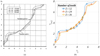 |
Fig. 14 Adjacent roller location characteristic curve according to (a) Kim & Johnson (parameter ξ) [17] (b) CDEM (parameter γ). |
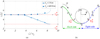 |
Fig. 16 ASA driving sprocket (a) example of roller location (b) tight and slack side of the profile. |
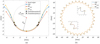 |
Fig. 17 Comparison of ASA, NFmax and NFmin profiles: (a) in the local profile coordinate system, (b) for a whole sprocket (31 teeth double pitch sprocket). |
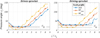 |
Fig. 18 Pressure angle ϕi for driving and driven sprocket. |
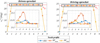 |
Fig. 19 Articulation angle for the driving and driven sprockets. |
ϕtp|A,B without friction correction for ASA, NFmin and NFmax tooth profiles.
Constants K and K' for NFmax, NFminand ASA.
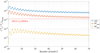 |
Fig. 20 Limit tension ratio in stable working conditions for industrial profiles. |
4.2 Cycling profile, definition and preliminary results
The three Cycling Profiles proposed (Fig. 21) are denoted CP1, CP2 and CP3 (see full definition in Appendix C). The definition of their geometry is based on the NFmin and NFmax ones (Appendix B). Compared to the industrial profiles (see Tab. 9), the Cycling Profiles exhibit smaller values of K (Tab. 10). Profile CP1 has the smallest K' parameter of all the tested profiles and will therefore tend more rapidly to its limit pressure angle ϕtp (∞) = K. Parameter K constitutes the limit value for an infinite number of teeth while parameter K' characterises how fast ϕtp tends to K for high Z (see Fig. 22). Profiles NFmin and CP3 show similar pressure angles. Profile CP2 has the smallest ϕtp for all the numbers of teeth tested. Below 15 teeth, profile CP3 has the biggest pressure angle. Its value then decreases toward that of CP2, leaving the NFmin and CP3 profiles with the highest ϕtp above 17 teeth.
As prescribed by equation (5), all the profiles show increasing ϕtp with the number of teeth Z. Profiles NFmax and ASA show the larger ϕtp which is consistent with their high limit tension ratio in stable working conditions (see Fig. 20). Despite the different K and K' parameters, the tooth profile hierarchy is usually respected as ϕtp ordering of the tooth profile families (i.e., ASA, NFmin, CP1, etc.) is similar regardless of the number of teeth (e.g., profile CP2 always has the smallest pressure angle, profile ASA always has the biggest). The only exception is the profile CP1 whose curve crosses those of NFmin and CP3 at about Z = 17 teeth. Due to its smaller K' parameter, it tends to reach its limit value more rapidly than the others. Consequently, its ϕtp is bigger than those of NFmin, CP2 and CP3 at Z = 10 but almost catches with CP2 at 70 teeth. The pressure angles of all the Cycling Profiles are smaller than those of the NFmin one (except CP1 for small numbers of teeth). They should therefore be able to withstand small tension ratios. The evolution of the limit ratio in stable working conditions is shown in Figure 23 (calculated with a friction correction of |δ (∞) | = 5 °). As expected, the low ϕtp values for the Cycling Profiles allow reaching small limit tension ratios in stable working conditions.
Figure 23 shows that only the NFmin and CP1,2,3 profiles can be used in track cycling applications (paper example of track cycling conditions shown with the red line) as the limit ratio is too high for both NFmax and ASA. Based on this assessment, and to study the influence of profile geometry on track cycling drives, NFmax and ASA profiles are removed from further study.
For CI = 300Nm, all the profiles show a maximum contact force at about 2000N (see Fig. 24). This value decreases to about 400 N for the second tooth (ζ/αI = 2). The decrease continues causing the final teeth (closer to the slack strand) to bear almost no load (Pi = 1.6Nat ζ/αI = 5). The same phenomenon is observed in link tension where almost no load is carried after ζ/αI = 4. Considering energy efficiency, tooth profiles with low ϕtp (e.g., profile CP2) result in more roller displacement. However, these displacements are performed with lower forces as the decreasing slopes are steeper. On the contrary, with a higher ϕtp value, the rollers undergo less displacement but the loads are higher. Therefore, it is not possible to easily assess which profile will result in the best efficiency, more in dept analysis must be carried on.
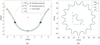 |
Fig. 21 Comparison of NFmin and Cycling profiles: (a) in the local profile coordinate system, (b) for a whole sprocket (Z = 15, p = 12.7 mm). |
Constants K and K' for cycling profile definition.
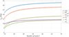 |
Fig. 22 Evolution of ϕtp with the number of teeth. |
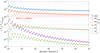 |
Fig. 23 Limit tension ratio in stable working conditions for the defined profiles, dotted red line for the current transmission from Table 3. |
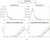 |
Fig. 24 Link tension, contact force and roller location for 60|15, slack=11%, CI = 300N . m, rear cog. |
4.3 Influence of chainring tooth profile, efficiency calculation and experimental comparison
Three chainrings from the market (denoted Chainring 1, 2 and 3) are compared, using the test rig, to the Reference chainring. All the tests are performed at Loading Condition LC1 (see Tab. 3) using a 60|15 drive configuration. A 15 tooth Reference rear cog was used for all tests. Parameters of the chains used corresponded to Table 2 with 100 links (see Fig. 25). The drive centre distance was again set to obtain a strand deflection under 1 kg mass of ≈20 mm. Slight differences in tight strand deflection were observed between chainring tooth profiles for a given centre distance L. Therefore, each drive was set with its specific centre distance to obtain the required tension setting (the values of L obtained ranged from 384 to 386 mm).
Manual interventions had to be performed on the test rig between the trials of the different chainrings. Due to these interventions, sensor offsets were modified causing the magnitude of total losses measured by the test rig to be different for each chainring. However, the Reference chainring was tested after each intervention. Therefore, a test with the Reference chainring is available for each chainring tested (i.e., Chainring 1, 2 and 3) in the same test rig conditions. Consequently, the results are given directly in Figure 26 relatively to the reference case (Reference chainring and rear cog). The difference ΔP corresponds to the losses obtained with a given chainring compared to those obtained with the Reference one.
As before, tests were performed in sessions of 25 min with measurements at 5, 15 and 25 min. Each comparison with the Reference configuration was carried out on 12 measurements (4 sessions of 3 measurements). The minimal and maximal values as well as the standard deviation are indicated in Figure 26.
The measured ΔP are negative, suggesting better efficiency with the tested chainring than for the reference case (Reference chainring and rear cog). However, all ΔP are included in the standard deviations. Therefore, the tests concluded that there were no significant differences between the three chainrings tested and the Reference one.
Except for the Reference tooth profile (denoted “Ref” in Fig. 27), the precise 2D geometries of the chainrings tested (Chainrings 1, 2 and 3) are not known by the author. To perform comparisons with the model results, the influence of the chainring tooth profile is assessed by testing the four profiles able to withstand track cycling constraints: NFmin, CP1, CP2 and CP3 (Sect. 4.2). The calculations are performed for LC1 (see Tab. 3) using the drive parameters given in Table 2 for 60|15 drive. The chain parameters can be found in Table 5 with 100 links. Drive efficiency as well as relative losses ΔP compared to the reference case are given in Figure 27. The intervals obtained using case A and case B are represented. For the relative losses, intervals [ΔPmin, ΔPmax] (see Fig. 27) are calculated assuming that cases A and B could occur indifferently for each configuration (see Eq. (6)).
 (6)
(6)
with:
Pref|A,B, the dissipation obtained with the Reference geometry for case A or B.
Pprofile|A,B, The dissipation obtained using the tested profile (NFmin and CP1,2,3) for case A or B.
The drive efficiencies predicted by the CDEM are identical for all the chainrings tested. Consequently, the ΔP values are negligible and included in the [ΔPmin, ΔPmax] intervals. Therefore, the model also concluded that the chainring tooth profile had a negligible effect on drive efficiency.
The CDEM can be used to explain the similar efficiencies for all the chainrings tested. Indeed, the computed losses are split between roller and meshing losses and between the chainring and the rear cog contribution. The proportions obtained for a CP1 chainring are presented in Figure 28 (j = I and II for the chainring and rear cog, respectively). Losses due the roller motion are denoted ‘roller’ while those due to meshing are denoted ‘mesh’.
First, it is observed that the total predicted losses are slightly higher for case B than for case A (4.81 W and 4.59 W, respectively). This was expected considering the less favourable hypotheses of case B. Meshing losses are caused by parameters depending on the global kinematics: tight strand tension Tt, pitch angle αI,II, etc. They are therefore identical for all the chainrings. Thus, changing the chainring tooth profile influences only the losses attributed to roller motion at the chainring. However, results show that this loss type contribution represents less than 1% (both for cases A and B). In these conditions, the negligible influence of chainring geometry seems consistent. This low proportion of roller motion related losses is due to the low-tension ratio (about 6.2e−3) resulting in small roller motion. Moreover, this motion occurs under moderate loading due to the rapid decrease in both link tension Ti and contact force Pi undergone using track Cycling Profiles.
The remaining proportions show that meshing losses are by far the greatest contributor in this loading condition. 18% of the losses are due to the chainring meshing losses while between 75 to 78% are caused by the rear cog meshing losses. This difference between chainring and rear cog meshing are directly related to the pitch angle αI,II [1,5,6]. Indeed, the rear cog pitch angle is significantly higher than the chainring one due to its smaller number of teeth (αI = 24° and αII = 6° in this example), resulting in a greater sliding distance. The results also show that roller losses at the rear cog are more significant than those at the chainring.
No significant influence of the chainring geometry was reported on the test rig measurements. Although direct comparisons using the tested tooth profile geometries could be performed, analysis of the model results prove that the chainring geometry is not a significant parameter under the loading condition tested. The CDEM prediction therefore seems correct.
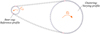 |
Fig. 25 Transmission used for chainring profile influence tests. |
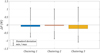 |
Fig. 26 Test rig measurements for the three chainrings tested relatively to the Reference case. |
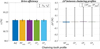 |
Fig. 27 Influence of chainring tooth profile according to the CDEM predictions. |
 |
Fig. 28 Loss contributions for the 60|15 drive, LC1, CP1 chainring and Reference rear cog. |
5 Conclusion
This article is devoted to the study, both numerical and experimental, of track cycling transmissions and the use of the results to identify the key parameters influence on their efficiency. To this end, a test rig dedicated to track cycling transmissions, including the chainring, rear sprocket and chain, was built. Its numerical counterpart, the CDEM [12], is a 2D quasi-static model that calculates the transmission efficiency induced by the kinematics of the chain as well as the local displacement of the roller on the profile of the chainring and rear sprocket teeth. The combined study of these two tools makes it possible to draw significant conclusions about the key parameters of cycling transmission:
The model and experimental data show that the tension ratio has a major influence on transmission efficiency. The experiment set the optimum strand deflection at 20 mm.
For a fixed gear ratio, increasing the number of teeth is beneficial for efficiency. This effect is already shown in the literature [6], but it is confirmed in the present study.
The experimental study on misalignment showed no significant difference with the perfect transmission. This validates the use of a 2D model for accurate predictions.
The study of sprocket profiles shows that their influence is very limited. The movement of the rollers on theses profiles, included in the calculation of the model, has only a limited influence on the losses in relation to meshing. However, the very small differences between cyclists in the track cycling race make this a possible source of optimization.
The experiments carried out on the influence of lubricants show that their proper use can have a major impact on transmission performance. The tests have shown that there is a possibility to improve the efficiency to more than 2 W using the right lubricant with the correct process of degreasing and application. The solid wax lubricants showed the best improvements. The durability of the lubricants was not tested, as the track cycling races are mostly short (<1 h) and in indoor conditions.
The model, which proved to be consistent with the experimental comparisons made, is intended as an aid to optimising cycling transmissions. All the results presented have been calculated using a single coefficient of friction. The model can break down the contribution of each interface (axle/brush, brush/roller and roller/profile), enabling highly localised optimisation. Its very low calculation time will also enable the various optimisation parameters to be investigated. To do this, a Design Of Experiment (DOE) built from it will be able to identify the main parameters responsible for the cyclist's performance. Finally, it should be borne in mind that, until now, all the calculations and experiments have been carried out under steady state conditions (constant torque and speed), which could find its limit in a sprint race, for example, where these conditions can vary rapidly.
Acknowledgments
The authors would like to thank Jean-Christophe PERAUD and Christophe CLANET for their support during the study as part of the THPCA2024 project.
Funding
This work is founded by INSA Lyon through a doctoral grant for the model part (development, calculation…) and by the THPCA2024 project supported by ANR (Grant No. ANR-2020-STHP2-000) for the experimental part.
Conflicts of interest
The authors certify that they have no financial conflicts of interest in connection with this article.
Data availability statement
Experimental data associated with this paper cannot be disclosed due to confidentiality reason. Model data (when displayed in this paper) will be made available on request.
Author contribution statement
Conceptualization, Gabriel Lanaspeze and Martin Best; Methodology, Gabriel Lanaspeze, Martin Best, Bérengère Guilbert, Jérôme Cavoret, Arnaud Duval, Lionel Manin and Fabrice Ville; Software, Gabriel Lanaspeze; Validation, Gabriel Lanaspeze, Martin Best, Bérengère Guilbert, Jérôme Cavoret, Arnaud Duval, Lionel Manin and Fabrice Ville; Formal Analysis, Gabriel Lanaspeze, Martin Best, Bérengère Guilbert, Jérôme Cavoret, Arnaud Duval, Lionel Manin and Fabrice Ville; Investigation, Gabriel Lanaspeze, Martin Best, Bérengère Guilbert, Lionel Manin and Fabrice Ville; Resources, Lionel Manin and Fabrice Ville; Data Curation, Bérengère Guilbert and Fabrice Ville; Writing − Original Draft Preparation, Gabriel Lanaspeze, Martin Best and Berengere Guilbert; Writing − Review & Editing, Gabriel Lanaspeze, Martin Best, Bérengère Guilbert and Fabrice Ville; Visualization, Gabriel Lanaspeze and Martin Best; Supervision, Bérengère Guilbert, Lionel Manin and Fabrice Ville; Project Administration, Fabrice Ville; Funding Acquisition, Lionel Manin.
References
- R.C. Binder, Mechanics of the Roller Chain Drive: Based on Mathematical Studies by R.C. Binder (Prentice-Hall, 1956), 204p. [Google Scholar]
- M.R. Naji, K.M. Marshek, Experimental determination of the roller chain load distribution, J. Mech. Des. Trans. ASME 105, 331–338 (1983) [CrossRef] [Google Scholar]
- B.H. Eldiwany, K.M. Marshek, Experimental load distributions for double pitch steel roller chains on polymer sprockets, Mech. Mach. Theory 24, 335–349 (1989) [CrossRef] [Google Scholar]
- M.D. Kidd, N.E. Loch, R.L. Reuben, Bicycle Chain Efficiency (Heriot-Watt University, Scotland, 2000) [Google Scholar]
- J.B. Spicer, C.J.K. Richardson, M.J. Ehrlich, J.R. Bernstein, M. Fukuda, M. Terada, Effects of frictional loss on bicycle chain drive efficiency, J. Mech. Des. Trans. ASME 123, 598–605 (2001) [CrossRef] [Google Scholar]
- C.J. Lodge, S.C. Burgess, A model of the tension and transmission efficiency of a bush roller chain, Proc. Inst. Mech. Eng. Part C J. Mech. Eng. Sci. 216, 385–394 (2002) [Google Scholar]
- S.P. Zhang, T.O. Tak, Efficiency estimation of roller chain power transmission system, Appl. Sci. 10, 1–13 (2020) [Google Scholar]
- M. Sgamma, F. Bucchi, F. Frendo, A phenomenological model for chain transmissions efficiency, IOP Conf. Ser. Mater. Sci. Eng. 1038, 012060 (2021) [CrossRef] [Google Scholar]
- A. Egorov, K. Kozlov, V. Belogusev, A method for evaluation of the chain drive efficiency, J. Appl. Eng. Sci. 13, 277–282 (2015) [CrossRef] [Google Scholar]
- R. Wragge-Morley, J. Yon, R. Lock, B. Alexander, S. Burgess, A novel pendulum test for measuring roller chain efficiency, Meas. Sci. Technol. 29, 075008:1–26 (2018) [CrossRef] [Google Scholar]
- G. Lanaspeze, B. Guilbert, L. Manin, F. Ville, Preliminary modelling of power losses in roller chain drive: application to single speed cycling, Mech. Ind. 23, 27 (2022) [CrossRef] [EDP Sciences] [Google Scholar]
- G. Lanaspeze, B. Guilbert, L. Manin, F. Ville, Quasi-static chain drive model for efficiency calculation − Application to track cycling, Mech. and Mach. Theory 203, 105780 (2024) [CrossRef] [Google Scholar]
- I. Troedsson and L. Vedmar, A method to determine the static load distribution in a chain drive, J. Mech. Des. Trans. ASME 121, 402–408 (1999) [CrossRef] [Google Scholar]
- M.R. Naji, K.M. Marshek, Analysis of sprocket load distribution, Mech. Mach. Theory 18, 349–356 (1983) [CrossRef] [Google Scholar]
- J.B. Spicer, Effects of the nonlinear elastic behavior of bicycle chain on transmission efficiency, J. Appl. Mech. Trans. ASME 80, 2 (2013) [CrossRef] [Google Scholar]
- N.E. Hollingworth, D.A. Hills, Theoretical efficiency of a cranked link chain drive, Proc. Inst. Mech. Eng. Part C J. Mech. Eng. Sci. 200, 375–377 (1986) [CrossRef] [Google Scholar]
- M.S. Kim, G.E. Johnson, Mechanics of roller chain-sprocket contact: a general modelling stragegy, in American Society of Mechanical Engineers, Design Engineering Division (Publication) DE 43 pt 2, pp. 689–695 (1992). [Google Scholar]
- M.R. Naji, K.M. Marshek, Analysis of roller chain sprocket pressure angles, Mech. Mach. Theory 19, 197–203 (1984) [CrossRef] [Google Scholar]
- ISO, ISO 606:2015; Short-pitch transmission precision roller and bush chains, attachments and associated chain sprockets. (2015). [Online]. Available: https://www.iso.org/fr/standard/61232.html [Google Scholar]
Contact and Structural Mechanics laboratory (http://lamcos.insa-lyon.fr/).
Cite this article as: G. Lanaspeze, M. Best, B. Guilbert, J. Cavoret, A. Duval, L. Manin, F. Ville, Identification of key parameter influence on efficiency of chain drive for track cycling − Preliminary results, 26, 21 (2025), https://doi.org/10.1051/meca/2025013
Appendix: A − Tooth profile definition
All tooth profiles considered in this manuscript are symmetrical. Therefore, only one half is defined. Then, the second one can be deduced by symmetry with respect to (O, y) (see Fig. A.1). NF tooth profiles are defined by the ISO 606 standard [31].
A.1 ASA tooth profile definition
The definition of the ASA tooth profile can be found in [1,18]. It is given as follows.
In Figure A.1, the ASA tooth profile is defined using four curve portions:
Between A and B, the first circle arc defines the tooth bottom. This arc is also called seating curve. Its centre coincides with the local origin O and its radius is strictly superior to the roller radius Rroller. Its parameters are: centre c1, radius R1, central angle θ1.
Between B and C, a second circle arc is called the working curve (centre c2, radius R2, central angle θ2.)
Points C and D are linked by a line called the straight portion.
Between D and E a last circle arc called the topping curve defines the tooth tip (centre c3, radius R3, central angle θ3.)
Curve portion parameters are given as functions of the sprocket pitch p, the number of teeth Z and the diameter of the roller to be used with the profile considered Droller. The pitch angle α = 2π/Z = 360 °/Z is also used as an intermediate variable. The radii Ri and central angles θi of each circle arc are summarised in Table A.1. Additional parameters needed to fully define the profile are given in Table B.1.
Radii Rii and central angles θi.
In [1], two main pressure angles values are given for the ASA profile:
-
First, the tooth pressure angle for new chain ϕnewchain. This angle is calculated assuming that rollers i − 1 and i are seated and that the roller/profile contact point (for roller i) lies at point B (see Fig. A.1).
 (7)
(7) The minimal pressure angle ϕmin is meant to account for rollers climbing the tooth flank. Its value is calculated still assuming rollers i − 1 and i to be seated. However, this time the contact point is considered to lie at point C (see Fig. A.1).
 (8)
(8)
These angles can be compared to the expression for ϕtp obtained using the CDEM, see Table 8.
Appendix: B. NF tooth profile definition
The profile shapes defined are symmetric. Therefore, only one half is defined and the second one is deduced from symmetry about (O, y), see Figure B.1. The defined half is given by two tangent circle arcs (to ensure slope continuity).
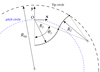 |
Fig. B.1 Definition of tooth profile with two circle sectors. |
Using two tangent circles arcs, these profiles are defined by four parameters (see Fig. B.1, Tab. B.2):
Parameters for NFmin and NFmax tooth profiles.
R1, and θ1 the radius and central angle of the first circle arc (tooth bottom).
R2, the radius of the second circle arc.
Rtip, the tip radius.
The centre of the first circle arc is the local origin O. The four parameters are functions of the sprocket pitch p, the number of teeth Z and the diameter of the roller to be used with the profile considered Droller. The pitch diameter  is also used as intermediate variable.
Appendix: C. Cycling tooth profile definition
The Cycling Profiles are defined similarly to the NF ones according to the parameters given in Table C.1. Compared to the NF profiles, the Cycling Profiles are only parametrised by the number of teeth Z. Therefore, their definition is only suitable for cycling applications (i.e., p = 1/2 " =12.7mm and Droller = 7.75mm).
Definition of the cycling profiles CP1,2,3.
All Tables
Comparison of the ΔP asymptote predictions between test rig measurements and CDEM predictions for LC1 and LC2.
Comparison of ΔP between experimental measurements and model predictions for different sprocket sizes.
All Figures
|
Fig. 1 Global CDEM algorithm, from [12]. With Ts,j:, αs,t,j:, nj, global variables, respectively slack tension, angle between a chain strand and the closest link with both rollers contacting spocket j (with j = I, II for chainring and rear cog) and contact number of rollers Ti, Pi, sc,r,i, κi, νi local variables, respectively link tension, roller contact force, curvilinear abscissa of roller, angle between the direction of the preceding link and the local x axis and the angle between the direction of the following link and the local x axis et k drive sub-position for efficiency calculation. |
| In the text | |
 |
Fig. 2 Nomenclature of a modern roller chain, from [12]. |
| In the text | |
|
Fig. 3 Track cycling efficiency test rig (a) general view (b) diagram. |
| In the text | |
|
Fig. 4 Illustration of the test protocol. |
| In the text | |
|
Fig. 5 Measurement of (a) tight strand deflection and (b) centre distance L. |
| In the text | |
|
Fig. 6 60|15 drives (a) slack=2% (b) slack=20%. Both figures have the same scale. |
| In the text | |
|
Fig. 7 Total power losses measured by the test rig for tension settings. |
| In the text | |
|
Fig. 8 Influence of tension setting: CDEM predictions. |
| In the text | |
|
Fig. 9 (a) 60|15 and (b) 53|13 drive, both with a looseness setting of slack=11%. Both figures have the same scale. |
| In the text | |
|
Fig. 10 Total power losses measured by (a) the test rig and (b) the CDEM for 60|15 and 52|13 drives for both Loading Conditions (LC1 and LC2). |
| In the text | |
|
Fig. 11 Transmission alignment scheme. |
| In the text | |
|
Fig. 12 Alignment results, Relative losses (W) compared to a well aligned transmission (a). |
| In the text | |
|
Fig. 13 Lubricants results, Relative losses (W) compared to manufacturer lubricant. |
| In the text | |
|
Fig. 14 Adjacent roller location characteristic curve according to (a) Kim & Johnson (parameter ξ) [17] (b) CDEM (parameter γ). |
| In the text | |
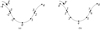 |
Fig. 15 Roller location coordinate for ASA profile according to (a) Kim & Johnson [17] (b) CDEM |
| In the text | |
|
Fig. 16 ASA driving sprocket (a) example of roller location (b) tight and slack side of the profile. |
| In the text | |
|
Fig. 17 Comparison of ASA, NFmax and NFmin profiles: (a) in the local profile coordinate system, (b) for a whole sprocket (31 teeth double pitch sprocket). |
| In the text | |
|
Fig. 18 Pressure angle ϕi for driving and driven sprocket. |
| In the text | |
|
Fig. 19 Articulation angle for the driving and driven sprockets. |
| In the text | |
|
Fig. 20 Limit tension ratio in stable working conditions for industrial profiles. |
| In the text | |
|
Fig. 21 Comparison of NFmin and Cycling profiles: (a) in the local profile coordinate system, (b) for a whole sprocket (Z = 15, p = 12.7 mm). |
| In the text | |
|
Fig. 22 Evolution of ϕtp with the number of teeth. |
| In the text | |
|
Fig. 23 Limit tension ratio in stable working conditions for the defined profiles, dotted red line for the current transmission from Table 3. |
| In the text | |
|
Fig. 24 Link tension, contact force and roller location for 60|15, slack=11%, CI = 300N . m, rear cog. |
| In the text | |
|
Fig. 25 Transmission used for chainring profile influence tests. |
| In the text | |
|
Fig. 26 Test rig measurements for the three chainrings tested relatively to the Reference case. |
| In the text | |
|
Fig. 27 Influence of chainring tooth profile according to the CDEM predictions. |
| In the text | |
|
Fig. 28 Loss contributions for the 60|15 drive, LC1, CP1 chainring and Reference rear cog. |
| In the text | |
|
Fig. B.1 Definition of tooth profile with two circle sectors. |
| In the text | |
Current usage metrics show cumulative count of Article Views (full-text article views including HTML views, PDF and ePub downloads, according to the available data) and Abstracts Views on Vision4Press platform.
Data correspond to usage on the plateform after 2015. The current usage metrics is available 48-96 hours after online publication and is updated daily on week days.
Initial download of the metrics may take a while.