| Issue |
Mechanics & Industry
Volume 26, 2025
Recent advances in vibrations, noise, and their use for machine monitoring
|
|
|---|---|---|
| Article Number | 20 | |
| Number of page(s) | 21 | |
| DOI | https://doi.org/10.1051/meca/2025012 | |
| Published online | 03 June 2025 | |
Original Article
Video-based operational modal analysis of slender mechanical structures with neutral axis estimation via barycenter calculation
1
Université Jean Monnet Saint-Etienne, IUT de Roanne, LASPI, UR,
42300
Roanne, France
2
Lab. Hubert Curien, CNRS UMR 5516, Université Jean Monnet, IOGS,
42000
Saint-Étienne, France
3
INSA Lyon, CNRS, LaMCoS, UMR5259,
69621
Villeurbanne, France
* e-mail: This email address is being protected from spambots. You need JavaScript enabled to view it.
Received:
21
June
2024
Accepted:
25
March
2025
Abstract
This paper presents an innovative adaptation of Operational Modal Analysis (OMA) by employing the concept of the barycenter to analyze dynamic behaviors in mechanical systems through video signal processing. Although this method is framed as a new contribution to the field of modal analysis, it is essential to recognize that its applicability is primarily confined to slender structures. Unlike conventional OMA methods reliant on numerical simulations or accelerometer measurements, this technique presents a non-contact, non-invasive measurement approach. It simultaneously captures multiple points across a wide field of view, ensuring robust measurements. The methodology was tested on a cantilever beam exposed to white Gaussian noise, with the beam recorded at 2048 frames per second to capture its dynamic response. The high-contrast environment facilitated image processing, while Laser Doppler Vibrometry (LDV) measurements served as a reference for validating the results. The proposed video-based OMA methodology demonstrated promising accuracy in capturing the system's dynamic behaviour by providing a more accessible and efficient alternative to traditional OMA techniques. Additionally, an analysis of the robustness of results concerning lighting conditions and video noise is conducted, along with a discussion on algorithmic complexity. Refinement of image processing algorithms and a broader application of this methodology to various mechanical systems and structures are proposed as important future objectives.
Key words: Video-based operational modal analysis / image processing / signal processing / barycenter / embedded beam
© J. Touzet et al., Published by EDP Sciences, 2025
 This is an Open Access article distributed under the terms of the Creative Commons Attribution License (https://creativecommons.org/licenses/by/4.0), which permits unrestricted use, distribution, and reproduction in any medium, provided the original work is properly cited.
1 Introduction
Operational Modal Analysis (OMA) serves as a cornerstone in understanding the vibratory behaviour of structures by identifying essential dynamic parameters such as natural frequencies, damping, and mode shapes without requiring external excitation [1,2]. This method leverages structures’ responses to ambient vibrations, providing a more natural and less intrusive modal analysis approach compared to traditional methods necessitating controlled excitation.
The spectrum of methodologies within OMA spans from time-domain approaches, such as stochastic subspace identification (SSI) [3], to frequency-domain approaches, such as the Least-Squares Complex Frequency (LSCF) method and the Least-Squares Frequency Domain (LSFD) which are fast and robust [4,5]. These techniques range in complexity, particularly in addressing coupled or overlapping modes, showcasing the extensive toolkit available depending on specific analytical needs. Simpler solutions, such as peak picking, present straightforward approaches for simpler analytical challenges, highlighting the versatility of OMA methods in various scenarios.
Historically, OMA measurements have predominantly used accelerometers [6], which are preferred for their cost-effectiveness and simplicity, but influence the mass of the structure and are limited by the number of measurable points. In pursuit of higher precision and quality, Laser Doppler Vibrometry (LDV) has been preferred [7], despite its higher cost and longer setup due to sequential measurements. This necessity has led to the emergence of video analysis methods, supported by high-speed cameras with global shutters and the potential future application using smartphones [8]. Nevertheless, this shift introduces considerable challenges, especially in signal dimensionality and data preprocessing, as the measured light intensity does not directly correspond to the physical position.
The exploration into video signal-based OMA focusses particularly on methods capable of characterising 3D movements using multi-camera setups. Some studies introduce techniques that enable 3D analysis using a single camera, primarily based on estimating the motion of a finite number of targets [9]. This motion is then projected on an operational modal basis using analytical [10] or finite element (FE) models [11]. A specific challenge in pre-processing is related to issues of projection and parallax, especially in cases of large movements. In the context of 3D structural analysis, Digital Image Correlation (DIC) stands out as a versatile technique capable of providing detailed deformation and strain measurements across an object’s surface. This method can be done using two cameras or one camera and another virtual one created, for example, through the use of mirrors [12] or other means. Despite its advantages in 3D analysis, including high spatial resolution and the ability to monitor complex deformations, DIC faces challenges such as high computational demands and sensitivity to lighting and surface preparation. Transitioning to 2D applications, DIC maintains its utility by allowing simpler setups and reduced computational load, making it an attractive option for studies requiring detailed surface analysis. The potential of DIC, especially when compared to point-based methods such as Laser Doppler Vibrometry (LDV) [13], highlights its applicability across both 2D and 3D modal analyses, providing a robust tool for capturing the dynamic response of structures.
For structures that can be accurately modelled in 2D, the computational demands are typically lower and spatial discretization of the object is not as stringent. These methods mainly examine the spatiotemporal gradient of light intensity, using techniques such as optical flow and subpixel measurement [14], which can be augmented with accelerometers or with a laser [15] for mid-frequency analysis. Digital Image Correlation (DIC) and Optical Flow are two key methods in precision measurement with distinct accuracy levels. DIC is especially notable for its precision, achieving measurements as fine as 1/10 to 1/100 pixels [16,17]. Phase-based methods, applied within the context of Operational Modal Analysis (OMA) for 2D structure modelling, present a sophisticated approach that uses phase information from video signals for motion detection [18]. Although these methods offer advantages in terms of precision and robustness against lighting variations, they are not without drawbacks. One significant limitation is their sensitivity to high-frequency noise, which can obscure the phase information critical to these analyses.
A particularly innovative method introduced in 2019 for OMA of beams focusses on estimating the barycenter intensity of light [19]. This straightforward yet effective approach necessitates particular conditions, such as uniform colour and cross section of the beam and stationary modes. Differentiating the camera acquisition frequency from the rolling shutter has yielded promising initial results, enabling the capture of modes at frequencies surpassing the Nyquist limit.
The main aim of this paper is to develop a methodology for theoretically estimating the minimum detectable motion, as well as its associated amplitude, using experimental parameters. This methodology is subsequently validated numerically, followed by experimental validation through modal analysis of a slender structure. This approach uses video analysis to estimate frequencies [20], damping, and deformation modes, based on the barycenter estimation technique to determine the position of the neutral axis of the beam. The straightforwardness and efficiency of this method, combined with the use of peak picking for frequency estimation and NEXT for damping evaluation, provide a complete approach for OMA. This opens the door to future applications, such as smart phone use and integration into active control systems [21], advancing toward more accessible and efficient structural health monitoring techniques. The beam was filmed at a rate of 2048 frames per second to capture its dynamic response. The high-contrast environment facilitated image processing, while LDV measurements served as a reference to validate the results obtained. However, the pursuit of precision in the estimation of modal parameters, particularly damping, unveils layers of complexity that merit thorough examination. Modal damping ratios are challenging to predict during the design process, but significantly influence structural dynamic behaviour. Consequently, estimating damping in vibrating structures using Operational Modal Analysis (OMA) is crucial, yet complex. OMA algorithms assume that input forces are stochastic, common in civil engineering structures. However, damping estimation can be influenced by many factors such as signal length [22] or input nonstationarity [23]. Accurately extracting modal damping, especially in the presence of residual harmonic content, requires careful selection of the bandwidth [24]. Moreover, understanding the effect of excitation on the amplitude of the vibration response is essential to avoid misinterpretation of changes [25]. In general, taking these parameters into account ensures reliable damping estimation in OMA for vibrating structures. The initial results of this video-based OMA methodology showed promise in accurately capturing the dynamic behaviour of the system, paving the way for a more accessible and efficient alternative to traditional OMA techniques.
The article is organised as follows: The first part presents the material and context, setting the stage for the study by outlining the foundational knowledge and specific conditions. The second part discusses methods and theory, elaborating on the techniques and theoretical approaches employed, ranging from image processing to damping calculation. The third part details the means of comparison of the obtained results, introducing criteria and methods such as the Modal Assurance Criterion Matrix and Spatial Registration used for validating the findings. The fourth part divulges the results, providing a comprehensive breakdown of the experimental parameters, frequencies, damping, and Modal shapes. The fifth part engages in a discussion about the implications of the results, considering computation time and the influence of various parameters, while also addressing the limitations and future prospects of the research. The article concludes with a sixth part that summarises the key findings and broader implications in the conclusion section.
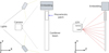 |
Fig. 1 Set up scheme for the two measurement: on the left, the video-based method under study; on the right, the laser-based method used for comparison. |
2 Material and context
The study presented in this paper focusses on a cantilever steel beam with dimensions 50 cm in length, 4 cm in width, and 0.2 cm in height under white Gaussian noise excitation. This serves as a model test case for the proposed video-based Operational Modal Analysis (OMA) methodology.
The test beam was painted white and set against a uniformly black background to create a high-contrast environment, facilitating the effectiveness of the image processing algorithms used in the methodology. The beam was firmly fixed at one end, left free at the other, and subjected to a white Gaussian noise input, a common type of random signal with equal intensity across all frequencies.
The beam was illuminated using a homogeneous light source to ensure consistent lighting conditions and to prevent the introduction of shadows or highlights that could potentially disrupt the video signal. High-speed cameras, which are capable of capturing fast-moving objects or events with a high frame rate, require intense and consistent lighting conditions for optimal performance. This is primarily due to their rapid shutter speed, which results in extremely short exposure times.
The schematic representation of the experimental arrangement is shown in Figure 1 and presents two concurrent methodologies, which focus on different sides of the beam. On the left, high-speed video footage of the beam was captured from a side profile using a camera that operates at 2048 frames per second. This high frame rate is crucial for accurately capturing the dynamic behaviour of the beam under excitation. The camera used for this study provided detailed measurements of the beam’s movement and variations in intensity. On the right, Laser Doppler vibrometer (LDV) measurements were performed on the beam independently of the video-based measurements. The LDV served as a reliable reference point for evaluating the precision of the results derived from the video-based Operational Modal Analysis (OMA).
The camera used for this study is an Optronis CP70-1-M / C-1000. The camera features a Lux1310 Global Shutter CMOS sensor with a resolution of 1,280 x 1,024 pixels. It provides a dynamic range of 53.7 dB and 12 bit A/D conversion. The obtained video is 8 bits, which means that it has 256 levels of intensity. The camera is positioned 500 mm away from the beam, with a focal length of 8 mm, which allows for a field of view of 526 mm.
The LDV measurements ensured high-precision point-wise velocity data, which is especially valuable for validating the video-based approach. The measurements taken with the LDV were conducted on one of the faces of the beam, not on the edge as is the case with the high-speed camera (Fig. 1). A mesh of 37 × 5 points, totalling 185 points, is used to conduct measurements with the LDV. It is important to emphasise that the spectral resolution of the laser vibrometer depends on the settings, and in this specific instance, it is 0.325 Hz. The spacially averaged periodogram obtained using every LDV points of the beam under white noise excitation is plotted in Figure 2.
Through this combination of materials and methods, an optimal environment | including a high-resolution camera, appropriate positioning, a high frame rate, as well as controlled environmental conditions | has been created to investigate the effectiveness of the proposed video-based OMA methodology. The following sections will detail the methodology, the analysis of the video and LDV data, and a comparison of the results.
3 Methods and theory
The section is divided into three subsections: the first will discuss image processing and all the necessary operations to obtain an image that is directly usable for subsequent analysis. Indeed, the image must be pre-processed to ensure it conforms to this condition. The second subsection will cover all the stages of signal processing that allow, starting from the pre-processed image, the extraction of inherent frequencies, modal damping, as well as the associated Modal shapes. The third subsection delineates the methodologies for comparing them to those obtained with the LDV.
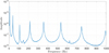 |
Fig. 2 Spacially averaged periodogram obtained using every LDV points of the beam under white noise excitation, to illustrate the estimation of natural modes with a state of the art methodology. |
 |
Fig. 3 Cropped Image of the beam before preprocessing. The image has a resolution of 1300 × 45 pixels. |
3.1 Image processing
The employed method necessitates a pre-processing step prior to obtaining the neutral axis of the beam. In fact, the method operates under the assumption that the beam should be illuminated against a dark background. Indeed, the position of the beam is determined on the basis of variations in intensity. Consequently, there is a need to somehow improve the contrast between the beam and the backdrop.
The image pre-processing steps are as follows:
Image cropping: The image is manually cropped to select only the relevant part. This step also reduces data volume and optimises computation time.
Mean filtering: Smoothing of the image using a spatial filter with a kernel
 . kernel 2 × 2 is employed to mitigate sensor-induced defects between adjacent pixels that can arise due to the Bayer matrix.
-
Contrast enhancement: the following transformation is used:
 (1)
(1)where Qi,j ∈ [0,1] is the intensity value of the input image pixel (i,j), Pi,j ∈ [0,1] is the intensity value of the corrected image pixel (i,j), µRoI and σROI are, respectively, the average and standard deviation of the background over a selected region of interest (ROI) of the image. This step helps to remove background noise from the image.
-
Image erosion: Erosion is one of the two fundamental operations in morphological image processing, the other being dilation [26]. Let I: E → ℝ be a greyscale image defined on a space E, and let B ⊂ E be a structuring element defined as a binary neighbourhood. The erosion of I by B is mathematically defined as:
 (2)
(2)where (i, j) are the coordinates of a pixel in the image, and (u, v) ranges over the relative positions of the structuring element B.
For each position (i,j) in the image, the operation computes the minimum of the image values I in the neighbourhood defined by the structuring element B centred on (i, j). This step allows for the removal of unwanted pixels that do not belong to the beam and that might have survived the contrast correction in the previous step. For the study, a vertical bar of size 1 × 5 is used as the structuring element to retain only the beam and eliminate spurious pixels.
-
Image dilation: Dilation restores the correct beam size. Using the previous notation, the mathematical definition of dilation is as follows:
 (3)
(3)The structuring element used for dilation is the same as the one used for erosion.
Figure 4 shows an example of the effects of image processing, where the histograms demonstrate how the background becomes homogeneous with a value of 0 after processing.
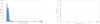 |
Fig. 4 Normalised histograms of an image: on the left, the raw image histogram; on the right, the histogram after preprocessing. |
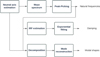 |
Fig. 5 Diagram showing the various processing steps implemented to achieve the OMA of the monitored structure. The steps are organized according to the objective targeted by the OMA and are detailed in Subsection 3.2. |
3.2 Extraction of modal properties
The steps to obtain natural frequencies, damping ratios, and mode shapes are described succinctly in the following subsections. The signal processing steps (Fig. 5) are as follows:
3.2.1 Neutral axis estimation
The neutral axis, where the beam experiences minimal deformation from bending, is the focus of this estimate.
With the assumption of small displacements, it is thus possible to equate a straight section with a column of the image, as the straight sections remain largely vertical in this specific case. Once preprocessing has been completed, the position of the neutral axis of the beam is estimated for each column of the image using a barycenter calculation. The intensity of the pixel (i, j) at time t, represented [t], is simply called pij.
For an image P:
 (4)
(4)
The barycenter g for each column j of the image P (j = 1,…, J) is defined as
 (5)
(5)
where
 (6)
(6)
In this formula, i represents the row index and pij is the intensity of the pixels in the row i and the column j.
This ensures that the calculation of gj, the barycenter of column j, reflects the weighted average of the pixel intensities over the rows with subpixel precision. The barycenter method offers a means to determine the absolute position within an image. However, in the subsequent spectral analysis, which is carried out column-wise, emphasis is placed on frequency bands around the modal frequencies, which results in overlooking the continuous or static components. As a consequence, the spectral analysis neglects any static deformation which, if necessary, can be added to the operational modal shapes after the analysis. This approach also ensures that the results of the NExT method are not influenced by static deformation. Now, considering a video consisting of N frames (n = 1,…, N), the barycenter for each column j is calculated in each frame n. The results are then collected in a matrix
 (7)
(7)
where
 (8)
(8)
represents the barycenters of column j across all frames. In other words, for each frame n, the vector g = [g1,⋯., gJ] represents the barycenters of all columns. When repeating this for all N frames, each gj forms a column vector describing the barycenter of column j over time. Thus, the matrix G is formed by concatenating the barycenters gj for all columns across all frames, and each vector gj corresponds to a column in the matrix G, effectively capturing the temporal evolution of the intensity barycenters across the entire video sequence.
An eigenmode is characterised by its natural frequency, damping ratio, and Operational Deflection Shape. These are the three parameters that are to be extracted from the video here.
3.2.2 Natural frequencies estimation
Calculating the mean spectrum of the signals contained in G, Equation [7], is useful for frequency estimation because it avoids having to do as much peak-picking as there are signals to study. The spatial average of power spectral densities (PSD) is defined as:
 (9)
(9)
where PW (gj) is the PSD of gj computed using Welch’s method. Natural frequencies are obtained by applying the peak picking method proposed by Liutkus [27] to  . The peak selection process follows an iterative procedure. Firstly, all local maxima in the spectrum are gathered, identifying potential peak locations. Next, convolution is performed with progressively larger window sizes, gradually smoothing the spectrum. At each smoothing step, the local maxima are retrieved and connected to previously obtained ones by increasing a selection criterion. The peak trajectories that survive this smoothing process represent significant peaks. Finally, the K highest eigen-frequencies of the first K modes correspond to the first K points in the selection criterion vector, thus identifying the K most important peaks in the mean spectrum.
3.2.3 Modal shapes reconstruction
If we denote
 (10)
(10)
the measurable transfer function between the excitation and the beam motion at the point of abscissa x. In the present case, the excitation, noted E(ω), is induced by the piezo transducer, which is assumed to be localized for simplicity. Gx(ω) therefore represents the temporal Fourier transform of the centroid matrix G presented in the previous section. This frequency response function can be represented by a K -degree-of-freedom modal model in the form:
 (11)
(11)
Where Ak represents the projection of the excitation onto mode k, normalized by the modal mass, and does not need to be estimated. It is sufficient to assume that this value is nonzero so that the mode ϕk can be observed at x. This hypothesis holds as long as the excitation is not applied exclusively at the nodes of the mode of interest. In our case, with the patch being close to the clamped end, we can reasonably assume that the lower modes of the structure will be observable.
We then assume that the system is lightly damped and that the natural frequencies are well separated. This simplifying hypothesis allows us to reduce the previous expression to the following form:
 (12)
(12)
where the corrective term ϵ, representing the contribution of the other modes, is neglected in the present case of the low-frequency behavior of a lightly damped bending beam. This simple approximation then allows us to estimate the mode shape at any point along the beam according to:
 (13)
(13)
Where Bk is a time dependant but spatially uniform gain that incorporates the amplitude of the excitation, which also does not need to be estimated. It is sufficient to consider this value as nonzero at the frequency ωk, so that mode k is effectively excited, as is guaranteed in our case by the use of white noise excitation.
3.2.4 Damping estimation
First, it is essential to recognise that the excitation in the system is stochastic in nature. This randomness necessitates careful consideration when selecting the appropriate calculation methods. The damping calculation is performed in two steps: the impulse response (I.R.) of each mode is estimated, and then a curve fitting between the envelope of the I.R. and a decaying exponential is conducted.
The Natural Excitation Technique (NExT) is an operational modal analysis method that estimates the impulse response (IR) of a structure by exploiting its natural vibrational responses induced by random environmental excitations, such as white noise [28]. The IR for every column j and mode k can be defined as:
 (14)
(14)
where:
 (15)
(15)
and:
 (16)
(16)
The mean IR is then:
 (17)
(17)
Once the IR are obtained, their envelopes are fitted for each mode with a decaying exponential equation  where λk is the damping coefficient of the mode k. The equation relating the damping coefficient to the damping ratio for a linear underdamped system (0 < ζ< 1) is given by [29]:
 (18)
(18)
3.3 Comparison criteria of the obtained results
The beam has been characterised using image and signal processing in the previous subsection. The obtained results are then be compared to those obtained with LDV, following exactly the same steps as those used for video analysis once the barycenter is obtained. Given Yj,k representing the Operational Deflection Shape obtained using the video at point j for mode k, Zj,l is then defined as the Operational Deflection Shape obtained using LDV at point j for mode l.
3.3.1 Modal assurance criterion matrix
The Modal Assurance Criterion (MAC) matrix is a widely used measure in modal analysis to assess the similarity between two sets of eigenmodes [30] and is defined as
 (19)
(19)
where the indices k and l represent vibration modes ranging from 1 to K, and j represents the abscissas in the matrices Y = [Yj,k] and Z = [Zj,l]. This method helps to determine to what extent the modes of a structure or system differ or resemble each other, based on Operational Deflection Shapes. An autoMAC matrix can also be defined to assess the quality and completeness of the obtained set of eigenmodes:
 (20)
(20)
autoMAC is used to evaluate the self-coherence of mode shapes. Its main function is to check if a mode shape is distinct and well defined, without interference from other modes.
3.3.2 Spatial registration
Comparison between video and laser vibrometer data requires spatial alignment of the signals. The application of MAC matrices requires that LDV and video estimations provide identically spatially discretised modes. However, this is not necessarily the case. The LDV focusses on the face of the beam, while the video captures its profile, complicating direct comparisons. Even disregarding these differing perspectives, matching the spatial resolution between the two data sets is highly time-consuming, as achieving the same level of detail demands substantial effort and resources. To address this, the application of Dynamic Time Warping (DTW) is proposed to align the data spatially, rather than temporally [31], allowing accurate comparisons despite these inherent challenges. DTW measures the similarity between two matrices by finding the optimal path that minimises the sum of distances between the corresponding points in the matrices.
Let Y and Z be the two matrices to be synchronised with Y ∈ ℝI×K and Z G ℝJ×K and J>I. The distance chosen to minimise is the squared Euclidean distance, defined as follows:
 (21)
(21)
Essentially, the goal is to find the pair (i,j) that minimises the sum of squared differences between the corresponding elements of Y and Z. In this study, the matrices Y and Z contain the Operational Deflection Shapes.
An accumulation cost matrix D of size I × J is constructed, where each element Di,j- represents the accumulated cost up to position (i, j) in the Y and Z matrices. The matrix D is defined as:
 (22)
(22)
with initial conditions:
 (23)
(23)
Optimal spatial registration is obtained by finding the path that minimises the sum of accumulated costs from D(I,J) to D(1,1). The variables sought to be determined are the indices i and j that define this optimal path.
However, rather than retaining all possible points along this path, only one optimal alignment point is kept for each row in Y. Specifically, this optimal point is the one that minimises the local distance d(Yi,Zj) between the row in Y and its corresponding point in Z. This ensures that each row in Y has a single, unique corresponding row in Z, thereby simplifying the alignment and avoiding redundant matches.
 |
Fig. 6 Pre-processing results: on the left, the raw image; on the right, the pre-processed version of the same image. The red crosses indicate the estimated barycenters. |
4 Results
Once preprocessing is completed, the methodology described in Section 3.2.3 is applied. Figure 6 shows the raw image obtained right after capture and the pre-processed image plus the estimated neutral axis of the beam.
Table 1 summarizes the effects of each preprocessing step on the normalized trace results for the crossMAC between the video and the LDV, highlighting their significance within the methodology.
Taken individually, it appears that contrast enhancement plays a predominant role in improving reconstruction quality, as evidenced by the significant increase in the normalised trace of crossMAC (Tr(crossMAC)/K) to 0.84, compared to only 0.07 for the other methods applied alone. This is primarily due to the need for the barycenter method to operate with a white object set against a consistently black background, which this step accomplishes.
However, the other pre-processing methods, although less impactful individually, also provide substantial improvements when combined. For instance, mean filtering combined with contrast enhancement reaches a Tr(crossMAC)/K value of 0.88, and applying all preprocessing steps yields the highest performance, with a normalised trace of 0.89. These results suggest that, while the preprocessing methods vary in their isolated impact, they are complementary and collectively contribute to optimising the reconstruction of the captured dynamics.
Influence of the preprocessing steps on the results obtained by displaying the normalised trace of the crossMAC between the LDV and the video. K is the number of reconstructed modes. Here, K = 6.
4.1 Frequencies and damping
Natural frequencies are obtained using the peak picking method (Fig. 7) described in Subsection 3.2.2. Peak picking enables the identification of the first 8 bending modes of the beam. The focus is on the first six bending modes to reduce computation time.
The results are summarised in Table 2. The absolute differences between the frequencies estimated from LDV and those obtained from the video are all below 0.5 Hz. The absolute differences between the damping estimated from the LDV and those obtained from video are all below 0.1%.
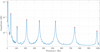 |
Fig. 7 Peak-picking performed on the averaged PSD derived from Welch’s periodograms. The results from the video processing display the identified peaks, which are highlighted with red circles. |
Comparison of natural frequencies (Hz) and damping ratios (%) between LDV and Video methods across various modes, including their respective differences (Diff.).
4.2 Modal shapes
The Modal shapes  are obtained from equation (13) described previously. The results are presented in Figure 8. The reconstructed Modal shapes are less smooth on the left side of each curve, likely due to the uncertainty related to the piezoelectric patch located on the pixels [80 290]. While the patch may influence the barycenter positioning, resulting in static errors, this alone cannot fully explain the observed discrepancies in the estimated amplitude of the dynamic motion. Further investigation is needed to determine whether the piezoelectric patch exhibits vibration or a more heterogeneous luminous appearance compared to the beam, as these factors may contribute to the observed artefacts more than the influence of the mode order. Indeed, the contrast between the patch, which conceals the edge of the beam, and the background is not sufficient to allow for an accurate reconstruction of the modes at this specific location. The results indicate that the experimental results agree well with the theoretical expectations for a cantilever beam.
Given the length of the beam and its observation over 1190 pixels, each pixel is estimated to represent a square of approximately half a millimeter on each side (0.45 mm). Then, the maximum displacements for each Modal shape have been estimated once the different Modal shapes are obtained. Table 3 shows the motion amplitude corresponding to each mode. A maximum displacement of up to approximately three-quarters of a pixel in amplitude is achieved for the first mode, and displacements in the order of hundredths of a pixel for the sixth mode.
This method, based on the correlation between two consecutive images, can measure displacements with a precision of 1/10 to 1/100 of a pixel, ensuring detailed and reliable measurements [16,17].
Once the Modal shapes have been obtained, the spatial registration of the two measurements is performed (see Fig. 9) to calculate the different MAC matrices.
The autoMAC matrices of the video and laser vibrometer are first computed. The results are presented in Figure 10.
The off-diagonal values for each of the autoMAC matrices are below 0.05 (5%), indicating that the eigenmodes can be considered orthogonal.
Subsequently, the cross-modal assurance criterion (crossMAC) matrix is computed between the shapes captured in the video and those measured by the laser vibrometer signals, and it is shown in Figure 11.
In the context of analysing a beam with a uniform profile, it is assumed that its mass is evenly distributed.
The LDV serves as a reliable benchmark for this analysis because it is essential to have a reference standard that does not alter the mass of the system, unlike the potential impact of using accelerometers. Finite element methods have been put aside in favour of this approach. Using the LDV as the benchmark, the first six bending modes of the structure can be precisely reconstructed from the video data, achieving a threshold of 0.8 in the cross Modal Assurance Criterion (crossMAC) matrix. This threshold indicates a high level of correlation between the measured and actual mode shapes, underscoring the effectiveness of using LDV as a reliable ground truth in dynamic system analysis.
Maximum estimated displacements of each mode.
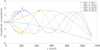 |
Fig. 8 Modal shapes obtained from video measurements. The amplitude of each mode is respectively normalized by its spatial effective value. The phase of each point is referenced relative to that observed for the free end of the beam, so that the shape remains real. |
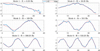 |
Fig. 9 Modal shapes after spatial registration. |
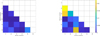 |
Fig. 10 autoMAC of the two measurement methods: on the left, the autoMAC from the video; on the right, the autoMAC from the LDV. Both autoMACs share the common scale on the right. |
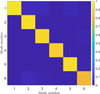 |
Fig. 11 crossMAC between the eigenmodes coming from the video and the eigenmodes coming from the LDV. |
5 Discussion
Considering the results obtained for the autoMAC of the various measurement methods, the proposed method appears to be capable of providing accurate results within the context of this study. This section will dive into several key aspects that offer another perspective on the quality and accuracy of the method. This section will begin with an analysis of the method’s computation time, focussing on its efficiency. Following this, the impact of noise on the results is examined, starting with the creation of synthetic images to simulate different noise conditions. Next, a theoretical estimation of the method’s precision is provided, considering various scenarios such as static cases, variations between successive images, and the inclusion of noise. The findings are then validated through both numerical simulations and experimental methods to ensure accuracy and reliability. Finally, this section concludes by discussing the study’s limitations, acknowledging any potential weaknesses and constraints in the approach.
Linear correlation coefficients for each parameter.
5.1 Computation time
Computation time, as outlined in complexity analysis, is critical for efficient algorithm performance, particularly in real-time applications. An efficient algorithm not only ensures timely results but also optimises resource utilisation.
Resolution is a major measurement parameter because it determines the number of pixels required to capture an image. It directly affects the processing time of the algorithms used. In this context, N represents the number of images in the video dataset, while I and J denote the dimensions of each individual image (with I referring to the number of columns and J to the number of rows). It can be shown (see Appendix A.1) that the complexity of the algorithm is O(I × J × N), which will be validated numerically.
A Monte-Carlo simulation will empirically validate this complexity by running multiple random trials, providing insights into average performance and robustness. The simulation will be conducted on a real-world video. The video has an initial size of 80x1000 pixels with 20480 frames.
For the influence of I (the number of rows), six different videos are created by modifying I from the original video. This is done by adding or removing lines on either side of each frame, using black pixels if I > 80. Similarly, to study the influence of J (the number of columns), J is modified by adding or removing columns and ten videos are created.
Figure 12 shows the linear influence of N, J, and I. These results are obtained through Monte Carlo simulation with 35 realisations.
The linear correlation coefficient r is calculated for each parameter to verify their linear influence. The results are presented in Table 4. The coefficients all have a value greater than 0.98, which confirms the linear influence of each parameter on the computation time.
The empirical validation of the algorithm’s complexity highlights the intricate dependencies of computation time on various parameters, ensuring a thorough understanding of algorithm performance under different conditions. These findings open opportunities to investigate additional elements that could affect the reconstruction of vibration modes from video data.
5.2 Influence of noise
The results obtained in Section 4 indicate that the reconstruction of vibration modes is achievable using a video camera. However, it is important to note that these results can be influenced by various measurement parameters.
Noise in video processing significantly affects the quality of the final output and the effectiveness of subsequent processing techniques. In the realm of digital video, “noise” refers to any unwanted or random variation in brightness or colour information, often manifesting as grainy specks or distortions in the image. This noise can originate from various sources, including sensor imperfections, low lighting conditions, or compression artefacts. The presence of noise can severely degrade the visual quality of a video, making it less appealing to viewers. In addition, noise can hinder the performance of algorithms used in video processing tasks such as object detection, tracking, and recognition. These algorithms often rely on clear and distinct visual features, and noise can obscure these features, leading to reduced accuracy and reliability. For such a study, synthetic images with known ground truth are created.
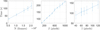 |
Fig. 12 Influence of parameters on computation time. |
5.2.1 Creation of synthetic images
To approximate experimental conditions, synthetic images are generated from a dynamic model of a cantilever beam subjected to white noise excitation. The natural frequencies and mode shapes of the beam are initially derived from solving the eigenvalue problem associated with its governing differential equations. For the five primary modes, the modal wavenumbers are explicitly defined as βk, k = 1,…, 5:
 (24)
(24)
For higher modes, i.e. k > 5, the wavenumbers are generated based on a more generalised formula:
 (25)
(25)
This model is subsequently used to derive the natural pulsations, which are formulated as:
 (26)
(26)
where E is the Young modulus of the material, I is the moment of inertia of the cross-sectional area, ρ is the density of the material and b and h represent the width and height of the cross-sectional area, respectively. Exploring modal characteristics, Modal shapes (ϕ) and modal masses (μ) are determined using modal wave numbers and beam length. The modal mass is determined by integrating the square of the Modal shape along the length of the beam, taking into account the density and dimensions These modal parameters are essential for constructing Frequency Response Functions (FRFs). Such FRFs offer a frequency-based depiction of the beam’s responses, guided by Modal shapes. After the frequency domain analysis, an extensive time domain response analysis was conducted to capture the beam’s behaviour over time. In practice, 1190 points were selected for reconstruction, mirroring the number of points in the actual video data set for a faithful representation of the beam’s behaviour. Symbolising one aspect of the analysis, Figure 13 presents a Bode magnitude diagram, offering information on the characteristics of the frequency response of the beam. This diagram serves as a visual representation of the synthesised FRFs, highlighting key frequency domains of interest.
In the following study, the focus will be on the first three bending eigenmodes.
In summary, this computational analysis integrates theoretical derivations with practical simulations, providing a holistic understanding of the dynamic behaviour of the cantilever beam.
In the process of transforming the analytic beam bending response obtained from the previous steps into a visual image, a series of specialised steps are employed. Firstly, the signal is subject to a variable amplification process, adjusted to meet the particular needs of the research. The amplified signal is then converted into a grey scale format with a defined precision level of 2−8, corresponding to an 8-bit image.
Following the precision setting, the visualisation step involves representing the signal that represents the beam with a certain thickness in the image. An accuracy of the beam thickness similar to the experimental conditions is chosen, which is 5 pixels. The value assigned to each pixel corresponds to the percentage presence of the beam in that specific pixel area. An example of such a reconstruction is plotted in Figure 14.
This approach goes beyond a simple binary representation in which a pixel is either entirely filled or empty. For example, if the beam covers half the area of a pixel, the value of that pixel would reflect the presence of 50%, with a value of  . These values apply only to the two edges of the beam. In the described ideal scenario, each pixel represents the beam’s presence with a dynamic range of 256 levels, assuming a “white” beam on a “black” background. This model allows for a precise representation of the beam’s spatial position. However, this assumes perfect contrast, which is rarely the case in reality. When the beam or background colours deviate from pure white or black, the expected dynamic range and precision are compromised.
The concept of brightness is crucial here. Brightness affects how light or dark an image appears, influenced by the actual luminance and the context within which it is viewed. Non-binary colours and varying luminance levels affect the perceived intensity of the beam, disrupting the linear relationship between the beam’s coverage and pixel values. This reduces the effective dynamic range, affecting the accuracy of spatial representation in practical applications. Studying its influence is of importance for precise imaging tasks, as it affects the accuracy of measurement and the interpretation of data.
After reconstruction, the Modal shapes are obtained using the proposed method as described in the article. The results, depicted in Figure 15, align closely with theoretical expectations, reflecting the first three bending modes of a cantilever beam, with eigenfrequencies closely matching those observed in real-world scenarios, thus reinforcing the validity of the images synthesised.
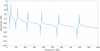 |
Fig. 13 Bode magnitude diagram of one reconstructed point of the beam. |
 |
Fig. 14 Example of image reconstruction for the vector g = [5, 5.25, 5.5, 5.75, 5.9, 6] where white corresponds to a value of 1 and black corresponds to a value of 0. The different shades of gray between white and black represent intermediate values. The blue crosses indicate the simulated positions of the neutral axis based on the vector g. |
5.2.2 Theoretical estimation of the method’s precision
The emphasis is on defining the accuracy of the utilised method, thereby suggesting the determination of the smallest detectable amplitude of modal movement and evaluating its reliability during video processing by the algorithm. The reasoning is divided into three subsections: the static case which formalises the relationship between pixel quantification in “greyscale” and spatial quantification related to barycenter estimation, the variations between successive images which illustrates the conditions favouring the detection of subpixel movement (referring to movement with an amplitude smaller than the previous spatial quantisation step), and the effect of additive noise allowing not only to get closer to reality while maintaining subpixel accuracy but also simplifying the problem.
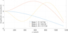 |
Fig. 15 Modal shapes obtained from synthetic images. |
5.2.2.1 Static case
In this first consideration, the focus is on the static case, which involves analysis based on a single image. The precision of the barycenter position can indeed be related to the bit depth (quantisation levels) of the image, but this relationship is not direct. Instead, it is related through the quantisation step sizes for the image and barycenter. Let µp be the mean value of the beam and βb the mean value of the background. The contrast can be defined as:
 (27)
(27)
The quantisation step size ∆R of the image can be calculated using the formula:
 (28)
(28)
where R is the number of quantification levels. ∆R is expressed in grey levels.
The quantisation step size ∆B of the barycenter can be calculated using the formula:
 (29)
(29)
∆B is expressed in pixels (or millimetres). Then:
 (30)
(30)
Figure 16 illustrates the relationship between the greyscale level of 11 successive pixels, chosen from a column of the image, because they contain the beam and the position of the barycenter.
In this example, R = 5 and C = 1, then ∆R = ∆B = 0.25. This means that each step in the greyscale value, which represents the brightness of a pixel, corresponds directly to a positional change of 0.25 pixels. Since the image resolution determines the smallest distinguishable change in intensity (quantised into five levels in this case), the corresponding positional precision of the barycenter is also limited by these increments. Therefore, a finer quantisation would lead to a higher positional precision, while a coarser quantisation would reduce it.
5.2.2.2 Variations between successive images
Extending beyond the static scenario, it is essential to examine how changes between consecutive images affect the detection of minor movements, characterized by a motion amplitude smaller than ∆R.
In the absence of noise, the detectability of the variation in the greyscale level p(n), n ∈ [0,N − 1], on a single pixel depends on the pair (mean, amplitude). If the variation is such that ∃q ∈ ℕ: p(n) ∈ [q∆R, (q + 1)∆R] (depicted in blue in Fig. 17), then the variation is annihilated by quantisation. In contrast, if ∃q ∈ ℕ: {p(n) < q∆R} = Ø, {p(n) > q∆R} = Ø, then the variation is bounded above by ∆R (depicted in red in Fig. 17).
This shows that the quantisation process can obscure small variations in the greyscale level, thereby affecting the detection and measurement precision in successive image frames. These observations highlight the importance of considering quantisation effects when analysing variations in greyscale levels over time, as they directly impact the accuracy and reliability of the measurements obtained.
5.2.2.3 Impact of noise on beam movement detection and measurement
Taking noise into account introduces significant nuances in the detectability and measurement of beam movements. Let us assume that there is an additive Gaussian noise with a mean of zero and a variance of  scaled in pixel quanta (1/R). Consequently, the background of the image adheres to a Gaussian distribution characterised by a mean µb and a variance
  . ypically, Gaussian noise falls within the interval [−2σb, 2σb], implying that the majority of noise values lie within this range. According to the empirical rule, approximately 95% of Gaussian noise values are contained within this interval.
If this level surpasses the quantification step ΔR (that is, if σb > 4), it is surprisingly demonstrated, firstly, that movement is unquestionably detectable for lower levels than the quantisation step exposed in the static case and, secondly, that its amplitude is no longer necessarily bounded above by the quantification step.
This phenomenon occurs because noise effectively “fills in” the quantisation gaps, making smaller movements detectable. This aspect will now be studied using frequency analysis.
With a probability of α, any peak observed in the amplitude spectrum of the barycenter position that exceeds a certain threshold η cannot be attributed to noise alone. This peak therefore arises from the complex addition of noise and the actual tonal component of the signal.
The threshold of interest, η, is defined as (see Appendix A.2):
 (31)
(31)
where σn represents the standard deviation of the noise in the barycenter position and N is the number of samples. This threshold ensures that peaks that exceed η are statistically significant and likely correspond to actual movements rather than random noise fluctuations. Thus, incorporating noise into the analysis improves the detection capacity and provides a more accurate estimation of the movement amplitude.
Moreover, equation (30) suggests an approximation of σn (spatial graduation) in terms of σb (grey-level graduation).
 (32)
(32)
The subsequent simulations and measurements will elucidate the order of magnitude relationship indicated by the static analysis.
Then:
 (33)
(33)
and:
 (34)
(34)
Consider an example where σb = 2 pixel quanta, μp = 200 pixel quanta, μb = 15 pixel quanta and α = 0.95, which corresponds to a confidence level of 95%. Thus, η ≈ 2.6 × 10−4 pixel.Hz−1/2, this means that any peak in the barycenter amplitude spectrum that exceeds this threshold has a 95% chance of not being noise and has its amplitude correctly estimated.
Thus, setting a high confidence level value prioritises stringent significance criteria, ensuring robustness in signal analysis and interpretation.
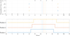 |
Fig. 16 Relation between the greyscale level and the position of the barycenter. The upper graph illustrates the normalized grey levels across various pixels after image preprocessing steps, where μp = 1 and μb = 0, for a quantification level of R = 5. The lower graph displays the respective beam positions. The dashed lines indicate the estimated centre of each beam using the barycenter method. |
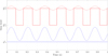 |
Fig. 17 Comparison of two time-domain signals. The dashed lines represent the true values, while the solid lines depict the discretised version. |
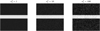 |
Fig. 18 Three images depicting a white beam against backgrounds with varying |

5.2.3 Numerical validation
The influence of additive noise and the study of its variance are crucial in this analysis. The assumption is that the pixel values of the beam follow a normal distribution  , where μp represents the mean pixel value of the beam, and
  is the variance. Similarly, the background is assumed to follow a normal distribution
  . The objective is to validate the results of Section 5.2.2 using simulations with synthetic images by varying the noise variance
  .
.
For this purpose, the mean pixel value of the beam (μp) is fixed at 225, and that of the background (μb) at 30.
Figure 18 illustrates different values of  . Noise is introduced before quantisation, necessitating the production of a distinct video for different values. This methodology allows for a detailed assessment of how beam brightness, in contrast to varying levels of background noise, influences the accuracy of bending-mode reconstruction.
This methodology is essential to evaluate the robustness of the reconstruction process in the presence of varying levels of noise. To this end, the indicators used are the diagonal terms of the crossMAC matrix defined in equation (19) and the ratio (ρ) between the estimated value of the standard deviation and the noise in the barycenter position defined as:
 (35)
(35)
where σn is the theorical value calculated from Equation [33] and  is estimated from the spectral baseline of the spectral density power spectrum of the barycenter position.
These indicators allow for the comparison, mode by mode, of each video for which noise has been varied, with an unnoised reference video whose reconstructed modes are presented in Figure 15.
The results obtained are plotted in Figure 19.
Two cases can be distinguished. When σb > 4, the conditions specified in the previous paragraph (5.2.2.3) are met, allowing the establishment of equations (31) to (34). The plot on the left numerically confirms the linear relationship described in equation (33), with  . In addition, the linear correlation coefficient is found to be 0.953. The right plot indicates that the estimation of σn is cautious, as the actual value is overestimated. In contrast, for σb < 4, the previous conditions no longer apply. It seems that σn remains above a specific limit as σb nears 0, and the estimation of σn is inaccurate.
In this specific case, all three modes are accurately reconstructed. A mode is considered accurately reconstructed if the diagonal terms of the crossMAC matrix exceed 0.8. This means that the amplitude of the three modes remains greater than the value of η when σb ∈ [0, 10]. The question now is to determine the threshold amount of noise that allows for proper detection and accurate estimation of these modes. Figure 20 shows the amplitude spectrum of the barycenter position in the case where σb = 0.
In this specific case, the amplitude of the third mode (the one at 117.7Hz) is approximately 0.008 pixels. Thus, the threshold for σb is determined when η = 0.008. Solving equation (34) for this η and α = 0.05 yields a maximum σb value of 91.2 pixels. Consequently, the three modes will be accurately detected and estimated if σb remains below 91.2 pixels.
To verify the maximum noise threshold values, another set of videos is used, where the amplitudes of the different modes are much lower than those studied in the previous case. The amplitudes of the three modes are obtained from the amplitude spectrum of the barycenter position. The mode amplitudes and the corresponding max values of σb are shown in Table 5.
The diagonal terms of the crossMAC matrix obtained are plotted in Figure 21.
The obtained limiting values of σb seem to match those estimated in the earlier table. Differences might arise because the threshold η is set based on a selected probability α, and the value of the diagonal element of the crossMAC, indicative of a satisfactory reconstruction, is also chosen arbitrarily (0.8 in this case).
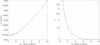 |
Fig. 19 Validation of the relationship between the standard deviation of the noise added to the images and that which disturbs the position of the beam’s barycenter. Left plot: estimated value of the standard deviation of the noise in the barycenter position. Right plot: |

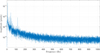 |
Fig. 20 Barycenter position amplitude spectrum of synthetic video where σb = 0. |
Amplitude of the three modes and the corresponding maximum value of σb (=σmax).
5.2.4 Experimental validation
In the conducted experiment, the noise variance is estimated due to a specific region of interest (ROI) in the greyscale image data of the entire video. The corresponding histogram is shown in Figure 22.
The beam is clearly separated from the black background. In fact, the beam shows values near 255 grey levels (μb = 255), while the background exhibits values in the range of grey levels [10, 30]. The noise variance is estimated to be around 13 (σb = 3.6) before image processing and μb = 18.1 in the experimentation.
For this study, the barycenter position amplitude spectrum is used for signal detection in noise (Fig. 23). The standard deviation σn is estimated with equation (33) and the associated threshold η is calculated using equation (34), with a confidence level of 95% (α = 0.05). The standard deviation  is estimated with the spectral baseline of the spectral density power spectrum of the barycenter position and the associated threshold
  is calculated using equation (31), with the same confidence level. In these conditions and with 10 seconds of acquisition (N = 20480), with σb = 3.6 pixel quanta, μp = 255 pixel quanta, and μb = 18.1 pixel quanta, then η = 2.6 × 10−4 pixels, which means that the minimum amplitude of motion that can be correctly detected and estimated is approximately 2.6 × 10−4 pixels. It is essential to note that the various frequencies previously estimated are not solely due to noise. The amplitude of the detected movement depends on the level of excitation within the given situation. Table 3 shows that the amplitudes of the different modes are greater than 0.045 pixels, which is consistent with the numerical validation ensuring good detection and accurate estimation of the modes when the movement amplitude of the mode is greater than 2.6 × 10−4 pixels.
Therefore, noise helps in estimating the amplitude more accurately, providing a value closer to reality than in the case without noise. It is important to recognize that although noise can be advantageous up to a certain point, too much noise can be harmful. When noise levels become excessively high, they can overpower the signal, rendering it difficult to obtain meaningful data or precise estimations. Therefore, it is essential to maintain an optimal noise level for accurate amplitude estimation.
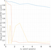 |
Fig. 21 Diagonal terms of the crossMAC matrix as a function of the noise standard deviation σb. The blue, red, and yellow curves correspond to the first, second, and third modes, respectively. |
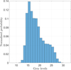 |
Fig. 22 Normalised histogram of a selected ROI corresponding to the background of a 20480 frames video. |
5.3 Limitations of the study
There are several limitations to the use of this method. The first limitation is the requirement for a beam to be illuminated against a dark background. Enhancing lighting conditions can lead to better contrast, potentially facilitating more accurate reconstruction of modes. It is important to note that the variance of background noise, which significantly impacts the quality of the image data, depends on several optimizeable parameters, with the quality of the camera being the foremost. By selecting a camera with superior sensitivity and resolution, and adjusting other factors like ambient light levels and lens quality, the background noise can be effectively minimised, further improving the contrast and thereby enhancing the potential for more precise mode reconstruction. A camera possessing a greater bit depth enhances precision by increasing the quantisation level R. The second limitation concerns the nature of the excitation applied to the beam. In this study, the use of white noise is essential for the simultaneous extraction of all vibrational modes of the beam. White noise, characterised by its uniform power spectral density across a wide range of frequencies, ensures that each mode is equally excited, facilitating their extraction. However, it is not necessary for every mode to be equally excited; the amplitude of the mode only needs to be higher than the noise level to ensure effective extraction. Additionally, the implementation of the Natural Excitation Technique (NExT) requires broadband excitation in order to estimate modal damping. This requirement is important because NExT is based on the response of the system to a wide range of frequencies to accurately identify the modal parameters. However, the need for broadband excitation can pose challenges in practical scenarios. It demands the generation of an excitation signal that spans a wide frequency spectrum, which might not always be feasible in controlled experimental setups. Moreover, ensuring that the excitation is uniform across the entire frequency range of interest is necessary, as any deviations can lead to inaccuracies in mode identification and analysis. Thus, the reliance on white noise and broadband excitation for the NExT method imposes constraints on the experimental setup and can affect the generalisability of the technique across different applications.
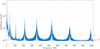 |
Fig. 23 Barycenter position amplitude spectrum example where R = 256 grey levels, α = 0.05, σb = 3.6 pixel quanta, μp = 255 pixel quanta and μb = 18.1 pixel quanta. The solid red line corresponds to the value of |

6 Conclusions
In this paper, an innovative video-based methodology for Operational Modal Analysis (OMA) has been presented, offering a comprehensive approach to characterising the dynamic behaviour of slender mechanical systems. The methodology successfully addresses some of the challenges faced by previous video-based OMA techniques, including the accurate extraction of displacement information from video signals and the minimisation of computational resources required.
Using a cantilever beam test case excited by white Gaussian noise, the effectiveness of the proposed methodology in capturing the modal properties of mechanical systems has been demonstrated. The high-speed video data was effectively analysed and compared to the ground truth provided by the laser Doppler vibrometer (LDV) measurements, highlighting the potential of video-based OMA as a viable alternative to traditional OMA techniques.
Key aspects such as computation time, parameter influence, and the effects of brightness and noise were thoroughly examined to evaluate the robustness and precision of this method. The analysis revealed a linear relationship between the number of frames, image dimensions, and modes, confirmed by Monte Carlo simulations, highlighting the method’s computational efficiency. Investigation of brightness and noise effects demonstrated that accurate vibration mode reconstruction is achievable.
Limitations include the need for optimal lighting to enhance SNR and white noise excitation for mode extraction. These constraints suggest room for improvement and adaptation in practical applications.
The advantages of the proposed methodology are numerous, including its non-contact, non-invasive nature, the ability to simultaneously measure multiple points over a wide field of view, and the reduced need for high computational resources. These benefits can significantly impact the field of OMA, making it more accessible and efficient for engineers and researchers from various industries.
Future work could focus on further refining the image processing algorithms to handle more complex and challenging real-world conditions, such as varying lighting or nonuniform backgrounds. Furthermore, the application of the methodology to a broader range of mechanical systems and structures will help validate its generalisability and effectiveness in different scenarios.
Funding
This research received no external funding.
Conflicts of interest
The authors declare no competing interests.
Data availability statement
The data that support the findings of this study are available from the corresponding author upon reasonable request.
Author contribution statement
Conceptualization, J.T., O.A., F.B., S.C., and H.A.; Data curation, J.T.; Formal analysis, J.T.; Funding acquisition, H.A.; Investigation, J.T.; Methodology, J.T., O.A., F.B., S.C., and H.A.; Project administration, H.A.; Resources, S.C. and H.A.; Software, J.T., S.C., and H.A.; Supervision, H.A.; Validation, S.C. and H.A.; Visualization, J.T.; Writing – original draft, J.T.; Writing – review and editing, J.T., O.A., F.B., S.C., and H.A.; All authors have read and agreed to the published version of the manuscript.
References
- J. Smith, A. Johnson, Operational Modal Analysis: Theory and Practice, Wiley (2019) [Google Scholar]
- R. Brincker, C. Ventura, Introduction to Operational Modal Analysis, John Wiley & Sons (2015) [CrossRef] [Google Scholar]
- Z. Guowen, T. Baoping, T. Guangwu, An improved stochastic subspace identification for operational modal Analysis, Measurement 45, 1246–1256 (2012) [CrossRef] [Google Scholar]
- J. Jaka, S. Janko, B. Miha, High frequency modal identification on noisy high-speed camera data, Mech. Syst. Signal Process. 98, 344–351 (2018) [CrossRef] [Google Scholar]
- B. Peeters, H. Van der Auweraer, P. Guillaume, J. Leuridan, The polymax frequency-domain method: a new standard for modal parameter estimation? Shock Vibr. 11, 523692(1900) [Google Scholar]
- L.F. Ramos, L. Marques, P.B. Lourenço, G. De Roeck, A. Campos-Costa, J. Roque, Monitoring historical masonry structures with operational modal analysis: two case studies., Mech. Syst. Signal Process. 24, 1291–1305 (2010) [CrossRef] [Google Scholar]
- D.M. Siringoringo, Y. Fujino, Noncontact operational modal analysis of structural members by laser doppler vibrometer, Comput.-Aided Civil Infrastr. Eng. 24, 249–265 (2009) [CrossRef] [Google Scholar]
- G. Klein, D. Murray, Parallel tracking and mapping on a camera phone, in 2009 8th IEEE International Symposium on Mixed and Augmented Reality, 2009, pp. 83–86 [Google Scholar]
- F. Renaud, S. Lo Feudo, J.-L. Dion, A. Goeller, 3D vibrations reconstruction with only one camera, Mech. Syst. Signal Process. 162, 108032 (2022) [CrossRef] [Google Scholar]
- S.P. Chaphalkar, S.N. Khetre, A.M. Meshram, Modal analysis of cantilever beam structure using finite element analysis and experimental analysis, Am. J. Eng. Res. 4, 178–185 (2015) [Google Scholar]
- F. Hild, S. Roux, Digital image correlation: from displacement measurement to identification of elastic properties – a review, Strain 42, 69–80 (2006) [CrossRef] [Google Scholar]
- L. Yu, B. Pan, Single-camera high-speed stereo-digital image correlation for full-field vibration measurement, Mech. Syst. Signal Process. 94, 374–383 (2017). [CrossRef] [Google Scholar]
- P.L. Reu, D.P. Rohe, L.D. Jacobs, Comparison of DIC and LDV for practical vibration and modal Measurements, Mech. Syst. Signal Process. 86, 2–16 (2017) [CrossRef] [Google Scholar]
- I. Tomac, J. Slavič, D. Gorjup, Single-pixel optical-flowbased experimental modal analysis, Mech. Syst. Signal Process. 202, 110686 (2023) [CrossRef] [Google Scholar]
- A.M. Wahbeh, J.P. Caffrey, S.F. Masri, A vision-based approach for the direct measurement of displacements in vibrating systems., Smart Mater. Struct. 12, 785 (2003) [CrossRef] [Google Scholar]
- V.V. Kibitkin, A.I. Solodushkin, V.S. Pleshanov, The effect of input parameters on the precision of DIC method, AIP Conf. Proc. 1623, 250–253 (2014) [CrossRef] [Google Scholar]
- X. Xiangyang, M. Yinhang, S. Xinxing, H. Xiaoyuan, Q. Chenggen, Experimental verification of full-field accuracy in stereo-dic based on the ESPI method, Appl. Opt. 61, 1539–1544 (2022) [CrossRef] [PubMed] [Google Scholar]
- Y. Yang, C. Dorn, T. Mancini, Z. Talken, G. Kenyon, C. Farrar, D. Mascareñas, Blind identification of full-field vibration modes from video measurements with phasebased video motion magnification, Mech. Syst. Signal Process. 85, 567–590 (2017) [CrossRef] [Google Scholar]
- H. André, Q. Leclère, D. Anastasio, Y. Benaïcha, K. Billon, M. Birem, F. Bonnardot, Z.Y. Chin, F. Combet, P.J.J. Daems, A.P.P. Daga, R. de Geest, B. Elyousfi, J. Griffaton, K. Gryllias, Y. Hawwari, J. Helsen, F. Lacaze, L. Laroche, X. Li, C. Liu, A. Mauricio, A. Melot, A. Ompusunggu, G. Paillot, S. Passos, C. Peeters, M. Perez, J. Qi, E.F. Sierra-Alonso, W.A. Smith, X. Thomas, Using a smartphone camera to analyse rotating and vibrating systems: feedback on the SURVISHNO 2019 contest., Mech. Syst. Signal Process. 154, 107553 (2021) [Google Scholar]
- S.Z. Khan, U. Ahmed, S. Qazi, S. Nisar, M.A. Khan, K.A. Khan, F. Rasheed, M. Farhan, Frequency and amplitude measurement of a cantilever beam using image processing: with a feedback system, in 2019 16th International Bhurban Conference on Applied Sciences and Technology (IBCAST), 2019, pp. 888–895 [Google Scholar]
- Z.-C. Qiu, X.-T. Zhang, X.-M. Zhang, J.-D. Han, A visionbased vibration sensing and active control for a piezoelectric flexible cantilever plate, J. Vibr. Control 22, 1320–1337 (2016) [CrossRef] [Google Scholar]
- G. Zini, A. Giachetti, M. Betti, G. Bartoli, Vibration signature effects on damping identification of a RC bridge under ambient vibrations, Eng. Struct. 298, 116934 (2024) [CrossRef] [Google Scholar]
- S. Kim, H.-K. Kim, Damping identification of bridges under nonstationary ambient Vibration, Engineering 3, 839–844 (2017) [CrossRef] [Google Scholar]
- P.-J. Daems, C. Peeters, P. Guillaume, J. Helsen, Removal of non-stationary harmonics for operational modal analysis in time and frequency domain, Mech. Syst. Signal Process. 165, 108329 (2022) [CrossRef] [Google Scholar]
- K.L. Ebbehøj, K. Tatsis, P. Couturier, J.J. Thomsen, E. Chatzi, Short-term damping estimation for time-varying vibrating structures in nonstationary operating conditions, Mech. Syst. Signal Process. 205, 110851 (2023) [CrossRef] [Google Scholar]
- J. Serra, Image Analysis and Mathematical Morphology: Ill., Graph. Darst. Vol. 1, Academic Press (1982) [Google Scholar]
- A. Liutkus, Scale-Space Peak Picking, Research report, Inria Nancy – Grand Est (Villers-lès-Nancy, France), January 2015 [Google Scholar]
- G.H. James III, T.G. Carne, J.P. Lauffer, The natural excitation technique (next) for modal parameter extraction from operating wind turbines, Technical report, Sandia National Labs., Albuquerque, NM (United States), 1993 [Google Scholar]
- N.S. Nise, Control Systems Engineering/Norman S. Nise, 6th international student version edn., John Wiley & Sons, Hoboken, NJ (2011) [Google Scholar]
- M. Pástor, M. Binda, T. Harčarik, Modal assurance criterion, Procedia Eng. 48, 543–548 (2012) [CrossRef] [Google Scholar]
- K.K. Paliwal, A. Agarwal, S.S. Sarvajit, A modification over Sakoe and Chiba’s dynamic time warping algorithm for isolated word recognition, Signal Process. 4, 329–333 (1982) [CrossRef] [Google Scholar]
Cite this article as: J. Touzet, O. Alata, F. Bonnardot, S. Chesné, H. André, Video-based operational modal analysis of slender mechanical structures with neutral axis estimation via barycenter calculation, Mechanics & Industry 26, 20 (2025), https://doi.org/10.1051/meca/2025012
Appendix A
A.1 Global complexity study
Complexity analysis of the method where I is the number of rows in the image, J is the number of columns in the image, K is the number of modes, and N is the number of images. The “cumulative complexity” field is obtained by taking the predominant complexity between the current row’s complexity and the cumulative complexity of the previous row.
A.2 Threshold of interest
Let X be the random variable that represents the amplitude of a peak in the amplitude spectrum of the barycenter position. Noise is assumed to be zero mean, additive, and white. The goal is to determine a threshold η such that:
P (X < η | H0) = 1 – α: probability that what is detected is only noise.
Under H0, X follows a Rayleigh distribution with parameter  . The cumulative distribution function (CDF) of a Rayleigh-distributed random variable X is given by:
 (A.1)
(A.1)
Setting this equal to 1 – α yields:
 (A.2)
(A.2)
So, the threshold η is:
 (A.3)
(A.3)
All Tables
Influence of the preprocessing steps on the results obtained by displaying the normalised trace of the crossMAC between the LDV and the video. K is the number of reconstructed modes. Here, K = 6.
Comparison of natural frequencies (Hz) and damping ratios (%) between LDV and Video methods across various modes, including their respective differences (Diff.).
Complexity analysis of the method where I is the number of rows in the image, J is the number of columns in the image, K is the number of modes, and N is the number of images. The “cumulative complexity” field is obtained by taking the predominant complexity between the current row’s complexity and the cumulative complexity of the previous row.
All Figures
|
Fig. 1 Set up scheme for the two measurement: on the left, the video-based method under study; on the right, the laser-based method used for comparison. |
| In the text | |
|
Fig. 2 Spacially averaged periodogram obtained using every LDV points of the beam under white noise excitation, to illustrate the estimation of natural modes with a state of the art methodology. |
| In the text | |
|
Fig. 3 Cropped Image of the beam before preprocessing. The image has a resolution of 1300 × 45 pixels. |
| In the text | |
|
Fig. 4 Normalised histograms of an image: on the left, the raw image histogram; on the right, the histogram after preprocessing. |
| In the text | |
|
Fig. 5 Diagram showing the various processing steps implemented to achieve the OMA of the monitored structure. The steps are organized according to the objective targeted by the OMA and are detailed in Subsection 3.2. |
| In the text | |
|
Fig. 6 Pre-processing results: on the left, the raw image; on the right, the pre-processed version of the same image. The red crosses indicate the estimated barycenters. |
| In the text | |
|
Fig. 7 Peak-picking performed on the averaged PSD derived from Welch’s periodograms. The results from the video processing display the identified peaks, which are highlighted with red circles. |
| In the text | |
|
Fig. 8 Modal shapes obtained from video measurements. The amplitude of each mode is respectively normalized by its spatial effective value. The phase of each point is referenced relative to that observed for the free end of the beam, so that the shape remains real. |
| In the text | |
|
Fig. 9 Modal shapes after spatial registration. |
| In the text | |
|
Fig. 10 autoMAC of the two measurement methods: on the left, the autoMAC from the video; on the right, the autoMAC from the LDV. Both autoMACs share the common scale on the right. |
| In the text | |
|
Fig. 11 crossMAC between the eigenmodes coming from the video and the eigenmodes coming from the LDV. |
| In the text | |
|
Fig. 12 Influence of parameters on computation time. |
| In the text | |
|
Fig. 13 Bode magnitude diagram of one reconstructed point of the beam. |
| In the text | |
|
Fig. 14 Example of image reconstruction for the vector g = [5, 5.25, 5.5, 5.75, 5.9, 6] where white corresponds to a value of 1 and black corresponds to a value of 0. The different shades of gray between white and black represent intermediate values. The blue crosses indicate the simulated positions of the neutral axis based on the vector g. |
| In the text | |
|
Fig. 15 Modal shapes obtained from synthetic images. |
| In the text | |
|
Fig. 16 Relation between the greyscale level and the position of the barycenter. The upper graph illustrates the normalized grey levels across various pixels after image preprocessing steps, where μp = 1 and μb = 0, for a quantification level of R = 5. The lower graph displays the respective beam positions. The dashed lines indicate the estimated centre of each beam using the barycenter method. |
| In the text | |
|
Fig. 17 Comparison of two time-domain signals. The dashed lines represent the true values, while the solid lines depict the discretised version. |
| In the text | |
|
Fig. 18 Three images depicting a white beam against backgrounds with varying |
| In the text | |
|
Fig. 19 Validation of the relationship between the standard deviation of the noise added to the images and that which disturbs the position of the beam’s barycenter. Left plot: estimated value of the standard deviation of the noise in the barycenter position. Right plot: |
| In the text | |
|
Fig. 20 Barycenter position amplitude spectrum of synthetic video where σb = 0. |
| In the text | |
|
Fig. 21 Diagonal terms of the crossMAC matrix as a function of the noise standard deviation σb. The blue, red, and yellow curves correspond to the first, second, and third modes, respectively. |
| In the text | |
|
Fig. 22 Normalised histogram of a selected ROI corresponding to the background of a 20480 frames video. |
| In the text | |
|
Fig. 23 Barycenter position amplitude spectrum example where R = 256 grey levels, α = 0.05, σb = 3.6 pixel quanta, μp = 255 pixel quanta and μb = 18.1 pixel quanta. The solid red line corresponds to the value of |
| In the text | |
Current usage metrics show cumulative count of Article Views (full-text article views including HTML views, PDF and ePub downloads, according to the available data) and Abstracts Views on Vision4Press platform.
Data correspond to usage on the plateform after 2015. The current usage metrics is available 48-96 hours after online publication and is updated daily on week days.
Initial download of the metrics may take a while.